
[Project] Train Delay Predictions
Published:
As this project was developed during my internship at DB Netz AG, the code can not be released. Furthermore, sensitive information is redacted.
Table of Contents
- Motivation
- Prerequisite
- Evaluation
- Approaches to Challenges of the Problem
- Data preparation and Analysis
- Analysis of Solution
- Conclusion and Outlook
1. Motivation
A high punctuality of trains leads to customer satisfaction. With the help of the project “PlanKorridore” (see official announcement ) traffic on busy rail routes are to be made more robust, thereby also improve the planning capabilities of the trains. A total of four particularly heavily congested corridors have been identified throughout Germany and defined as “Plan Korridore”.
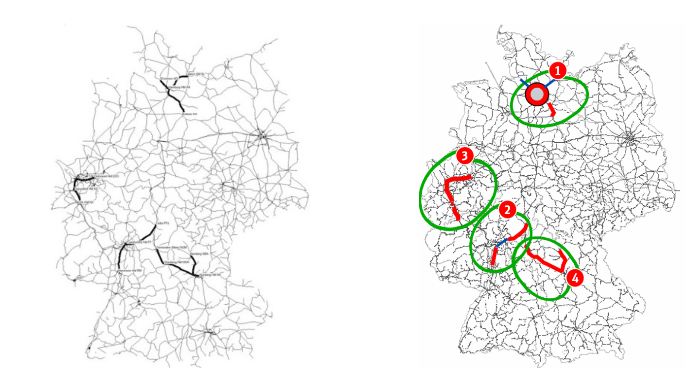 Fig: Plankorridore are 1. Hamburg, 2. Mannheim - Frankfurt - Fulda, 3: Köln - Dortmund, 4: Nürnberg - Würzburg
With the help of scheduling measures, trains running through planned corridors should remain on schedule or be made on schedule. Scheduling measures are, for example, a change of platform edge for a train with a door malfunction, an early turnaround of a train or even a rerouting of delayed trains via alternative routes.
The goal is not only to improve timeliness in the corridors, but also in the entire network. Because if there are delayed trains in these corridors the delay is propagated through the entire network due to various interactions. This leads to consequential delays in the entire network due to the large number of trains running through these corridors
2. Prerequisite
In the following section, we will further specify the delay prediction framework.
2.1 Description of the Problem
The requirement of the forecast is not to estimate a continuous value for the delay of a train, but the prediction of a delay of a train in a time interval (e.g. in the interval 1 - 3 minutes) - It is therefore a classification problem. Classes are defined as follows: [<1, 1-3, 4-6, 7-15, 16-30, 31-40, 41+]. The background for this is that for each class different proposals for scheduling measures were defined.
Another question we need to clarify is the time horizon of the prediction. As an example, let’s take the Fulda - Frankfurt - Mannheim corridor. If we forecast a very high delay in Mannheim after the departure in Frankfurt, skipping the train station at Frankfurt airport can not be performed. This is because we had to inform passengers about skipping this station in a reasonable time before the Frankfurt stop, so that they can take a replacement train from Frankfurt to the airport. As a rule of thumb, we say that we want to make predictions about the delay at the final stop 1 to 2 hours before entering the corridor.
2.2. Challenges of the Problem
Delay predictions are still a difficult task today. It is obvious that many external factors make prediction difficult, even impossible - there are, however, negative factors that we can include in the models. The first step to overcome such hurdles is to identify the problems.
2.2.1. Class Imbalance
We redact details of our dataset.

Severe delays occur only rarely, but these are the cases which are important for our problem. However, “naive” regression models will not be able to predict exactly such cases. Too low amounts of high delays cannot be learned by the model. Since the bulk of the data consists of low delays, the model will learn the patterns of low delays. Mathematically speaking, when training, the minimization of empirical risk is dominated by the high amount of low delays and thus the model will also predict this data better. This problem is also called “the long tail problem”.
The same problems arise when we convert the problem into a classification problem. The long tail problem gives us imbalanced classes.
2.2.2. Data Inaccuracies
Our data, as we discuss later in Section ???, consists largely of train running reports. While it is possible to infer information from train movements and possible patterns, many factors that lead to delay cannot be inferred from train movements. For example, because the available train running messages are macroscopic, conflicts on a track at a stop cannot be detected. From our train running messages, we cannot see which track a train is even entering and whether a track is occupied. We cannot map and predict various infrastructure conflicts and train dependencies from our data, although such conflicts play an important role. This would require microscopic data sets, which we do not currently have.
2.2.3. Localities
Dynamics that prevail on one route section can behave completely differently on another route section. Machine learning algorithms, however, try to draw information from all route sections and generalize it. It is obvious that the Frankfurt station stop behaves differently than the Gerolstein stop, which has little passenger volume. Such dynamics are essential in the development of models. One should also be aware that there is a trade-off between a uniform model, associated with lower computational load, and many small models that can represent the dynamics.
2.2.4. Flexibility of the Problem
The problem can be viewed from several angles: One approach would be to view the problem as a regression problem. One would predict the delay in seconds (or other time units) and then convert the delay to the appropriate classes.
It is also useful to follow a multiclassification approach. In multiclassification, one directly estimates the delay class for each observation rather than its delay in seconds.
Another approach uses the information from the relationship between classes to directly predict a class for each observation. The classes follow an order based on the height ̈he of the delay. Thus, for a misclassification it is relevant whether the error is two or three classes large. This approach is called ordinal classification or ordinal regression.

Why does flexibility now make the problem more difficult? It is not clear a priori which of these approaches is the best. So we have to understand, evaluate and compare 3 different approaches, and also the different models that exist for each approach.
3. Evaluation
3.1. Model Selection and Assessment
It is important to first of all keep in mind what exactly we want to achieve. We have exactly 2 different goals:
Model Selection: We want to be able to evaluate and compare the performance of different models in order to choose the best model in the end.
Model Assessment: We want to estimate the error of the final model on new data (generalization error).
The best practice is to split the available data into 3 parts: a training set, a validation set and a test set. The training set is used to train the model and the validation set is then used to evaluate the performance of the models and possibly try different hyperparameters. How to evaluate a performance or the error of models will be discussed in more detail. The best model, according to the selected metric, is taken in the end. This would be the Model Selections process.
 Fig: A possible split: 60% training data, 20% validation data, 20% test data.
The test set is used to estimate the generalization error of the best model. So one should leave this set untouched until one is done with the model selection.
3.2. K-Fold Cross-Validation
K-Fold Cross-Validation is a widely used method to estimate the expected generalization error. The method can also be used to get around the problem that data sets are too small for the “usual” split into training, validation and test set. In the end we have only 2 splits, a training set and a test set.
We first divide the data set into training data and test data, setting aside the test data. We again divide the training data into K approximately equal folds. Next, for the kth fold, we will train the model on the other K - 1 folds of the training data set and calculate the error on the kth fold of the training data set. Perform this procedure for k = 1,2,…,K. In the end, K prediction errors are obtained, and then the mean value is calculated. One can thereby compare different learning methods with different hyperparameters, where the goal is to minimize the mean value.
In the last step, the whole training data set is used to train the model with the found hyperparameters, which is our final model. Finally, the final model is evaluated on the set aside test data and gives us the generalization error.
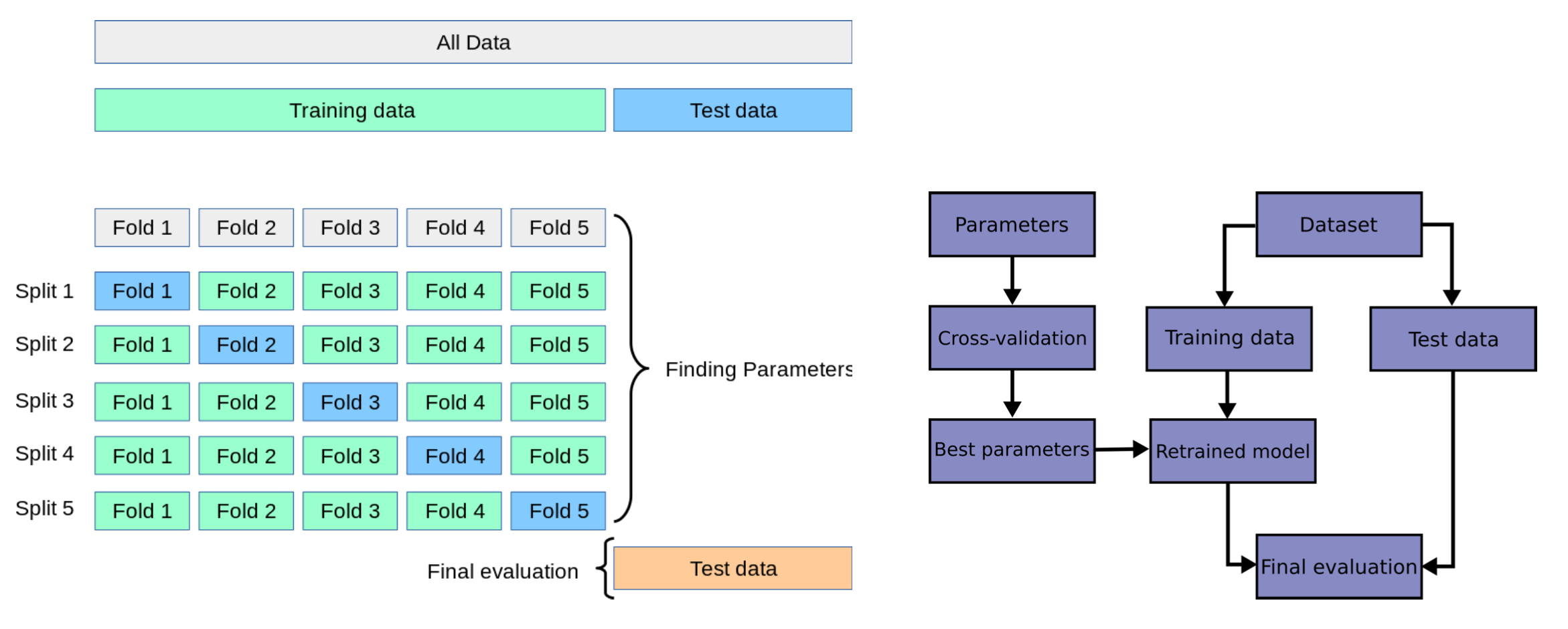 Fig: Example of a split for K = 5. Flowchart of CV.
3.3. Evaluation Metrics
The Confusion Matrix is a tool to visualize the performance of a model and to examine how it behaves in the individual classes. It can thus show problems with class imbalance.
 Fig: Illustration of a Confusion Matrix. It is easy to see that we cannot predict the class "not on time" ("nicht pünktlich"). It shows that our model is not suitable..
From Confusion, one can compute other metrics, especially important metrics for the analysis of individual classes.
 Fig: Illustration of a Confusion Matrix. It is easy to see that we cannot predict the class "not on time" ("nicht pünktlich"). It shows that our model is not suitable..
Precision: The precision can be calculated for each class. It is calculated for class j by dividing the correct predictions of class j by the total number of predictions for class j. Or stated informally: If the model predicts class j, how “certain” is the model?
Recall: The recall can also be calculated for each class. It is calculated for class j by dividing the correct predictions for class j by the total number of actual observations in class j. Recall, then, tells us what fraction of class j we correctly predicted.
F1-Score: The F1 score of class j is calculated by the harmonic mean value of precision and recall of class j of the model.
Macro F1-Score: The macro F1 score can now be used to evaluate the overall performance of the model by averaging the individual F1 scores. However, if one wants to evaluate the importance of the individual classes differently, one can introduce weights for the individual F1 scores. One choice for the weights is to take into account the number of observations in the classes:
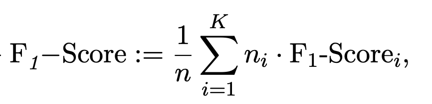
where n is the total number of observations and n_i is the number of observations in class i.
3.4. Baseline Models
Baseline models give us a reference to compare different models. We always need a reference to know whether the developed model is usable or not. The goodness of a model is always relative to the difficulty of the problem. It is difficult to evaluate how well our model performs, especially in our problem.
Naive Classifier: The simplest model in a classification is guessing. In a binary classification, we would have an average accuracy of 50%. Extended to a multiclassification with 7 classes, we get an average hit accuracy of 0.143 by guessing. However, since we have class imbalance present, we can use a new approach, which we call the naive classifier. The naive classifier takes into account the number of observations in the classes. Using the available data, we can estimate the class probability of class k estimated by

where n is the number of available observations. The naive classifier now classifies all observations x to the class with the highest estimated class probability, i.e.

In words: We classify each observation to the class with the most observations in the training set.
Relative Position: The naive classifier is a general model that can be taken as a baseline for any classification. The classifier does not process any information that is available in the context of the problem. For example, one would not classify a train that is 2 hours late as on-time at the next operating point just because there are more on-time trains than unpunctual trains. It is clear that the delay in the starting point plays a significant role in the delay in the ending point. We will use this information in the next “relative position” model. The relative position predicts for each observation the delay it has at the starting point as the final delay. The prediction is therefore relative to the delay at the starting point.
The “relative position” model is also used in the DB Navigator App (with some additional logic).
4. Approaches to Challenges of the Problem
4.1. Approach for the Imbalanced Data
There are 3 different ways to deal with class imbalance: Data-level approach, algorithm-level approach and a hybrid form. In the data-level approach, an attempt is made to balance the data set before a classification algorithm is used. In the algorithm-level approach, the imbalance of classes is taken into account in the structure of the algorithm, for example in the loss function. The last approach is a hybrid form of both.
In this project, we use Smote.
Smote: In the following, we will describe one of the best known forms of oversampling called SMOTE (Synthetic Minority Oversampling TEchnique). The idea of the method originates from handwriting recognition, where one creates new training data by rotating, flipping, and distorting, which has been successful in improving performance. We will now describe the method from the paper by Chawla et al. SMOTE generates new training data in a general way, it is not specific to only one application. New synthetic observations are created by performing operations not in the “data space” but in the “feature space”.
The minority classes are all oversampled in the SMOTE algorithm. Let us explain the procedure using one of the minority classes: Take an observation from the class and compute the k-nearest neighbors. Depending on how many synthetic observations one wants to create, neighbors are randomly chosen from the method. Now the difference between the feature vector (the observation) and the nearest neighbor is calculated. Now multiply the difference by a random number between 0-1 and add the result to the feature vector. This gives a random point on a line between 2 observations. This approach thus tries to generalize the decision space of the minority class.
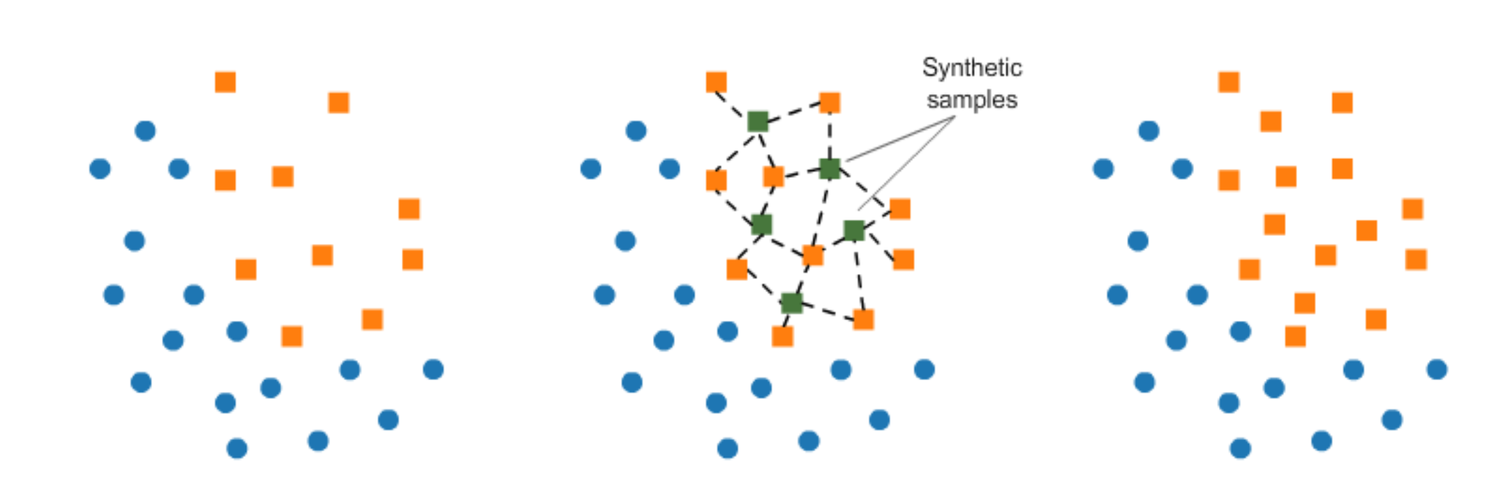 Fig: Example of a binary classification with 2 features.
4.2. Flexibility of the Problem
First, let’s explain in more detail how the ordinal classifier works, and then let’s explain the Stacking procedure and how it can use flexibility to its advantage.
4.2.1 Ordinal Classification
Ordinary classifications cannot use the information of the order for ordered classes. They assume unordered classes and classify accordingly. The class distance in case of misclassification is not taken into account and is penalized the same for each distance. The problem of ordered classes is also called ordinal classification or regression. But how can this information be used?
The problem is first partitioned from a multiclassification with K classes into k - 1 binary classifications. We assume that the ordinal attribute is denoted as A* with ordered classes V_1, V_2, …, V_K. A binary classification is defined for the first k-1 classes (i.e., for all but the last class). The i-th binary classification tests for each observation with attribute A* whether A* > V_i holds or not. One creates new data sets for the K - 1 binary classifications from the original data set. In the next step, one applies a binary classifier to each newly generated dataset, outputting the two class probabilities (rather than the class). Now, to make predictions for our original classification, one uses the predictions of the K - 1 binary classifiers:

To calculate the probability of the first and last class, we need only one classifier each, the first and last. The class with the highest probability is predicted. Empirical results can be found in the paper by Eibe Frank and Mark Hal.
Example: Define 3 classes. We now convert the multiclassification with 3 classes into 2 binary classifiers. After training the 2 binary classifiers, we can compute the probabilities of the original 3 ordered classes:
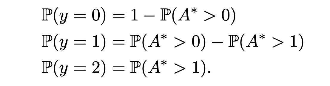
In our case, we would have 6 binary classification tasks.

4.2.2. Stacking
As we have already seen, there are very many machine learning algorithms, with different problem approaches that can be followed. The problem now is to test each of these algorithms individually and then select the best one based on a metric. Stacking now replaces this process by no longer having to “hand pick” an algorithm, but Stacking leaves this work to another Machine Learning algorithm. In fact, the algorithm no longer has to select a single model, but can actually combine several to make the best prediction.
Stacking is an ensemble technique that combines information from many different models to develop a new model. Simply put, Stacking obtains the output of each model from different machine learning algorithms that train different models. The collected outputs are then formed into a new data set. In the second step, this new dataset is then considered as a new supervised problem and a new machine learning algorithm finally solves the problem. The models in the first step are also called level-0 or base learners. The model in the second step that combines all predictions into one is called a meta learner or level-1 generalizer. The output of the base learner is then also called meta features, the new features for the meta learner.
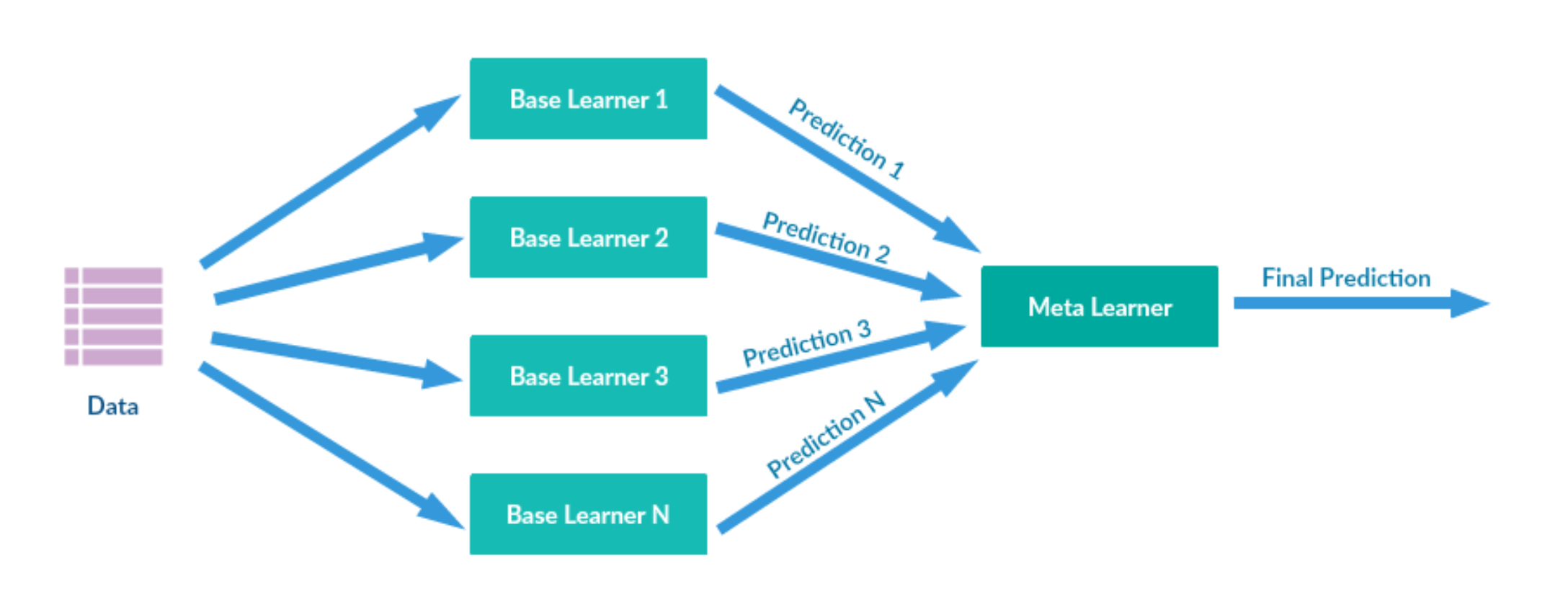 Fig: Simple sketch about stacking.
5. Data preparation and Analysis
An important component for a machine learning approach is a good data basis. It is essential to understand the data precisely and to cleanse it of erroneous or missing values. In the first part, we will explain how the data is collected and how the data is structured. In the second part, we will show examples of erroneous data and how we deal with them. In the last section, we analyze our cleaned data.
5.1. Data Basis
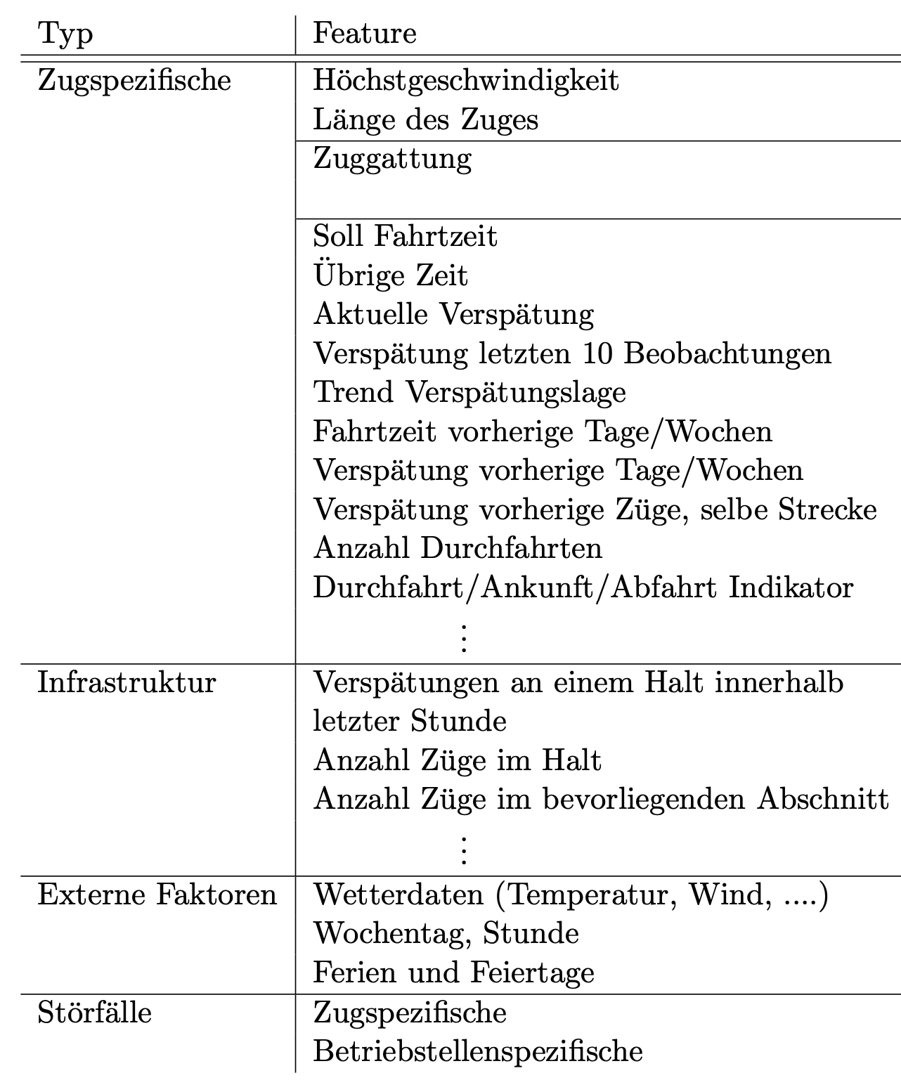
Train Running Messages: The largest part of our data consists of train running messages. These messages are generated by sensors located at the beginning and end of each train station. A train is now detected if it passes through a station, stops there or departs. For passages, the measured values of these sensors are interpolated so that only one time for the passage is indicated. Various key figures are created, whereby we will only use key figures that are important for a delay prediction in a certain way.
Train-specific key figures: Another data source gives us the train length (zl laenge), maximum train speed (zl vmax) and train type. The train type plays a particularly important role in the forecast, since a long-distance train behaves differently than a freight train, for example.
Incidents: If the travel time between two measuring points (sensors) is at least 90 seconds longer than the target travel time, a so-called lost unit is created. These must then be recorded with a reason for delay. The reasons originate from 55 cause groups (vuid), which in turn are divided into 9 super-groups.
Here, we will separate two different types of incidents. On the one hand, we have train-specific incidents, such as a drive malfunction on the vehicle, and on the other hand incidents specific to the operating site, such as a construction site. Train-specific incidents may extend throughout the entire train journey, which is why, if an incident occurs on the train, we record it at each additional measuring point for the train in question.
Holidays: Another data source gives us the school vacations and public holidays for each state.
Weather Data: The following key figures are taken into account: Temperature in Celsius, snow height, rain, new snow per hour, wind gusts, mean wind within one hour.
6. Analysis of Solution
In this part we will describe and evaluate our approaches.
6.1. Setup
We will first restrict the analysis to the corridor Fulda - Frankfurt - Mannheim, to the period from 01.07.2018 to 01.08.2019 and to long-distance trains only. We restrict ourselves to estimate the delay in Mannheim and include 2 stops before entering the corridor, i.e. 2 stops before Fulda.
To compare different approaches, we need to standardize the evaluation process for all approaches. We evaluate our results on the UE P, UEI, FFU (Fulda), and RM (Mannheim) starting points at arrival and departure, respectively, using the k-fold cross-validation method.
Splitting the Data: We have to keep one thing in mind when splitting the data: Days that are in the test set should not be in the training set. If we did not pay attention to this, we would not use true “unseen” days, because the model may be able to draw information from these days during training, but we would not have it in practice. Note that it can also be information that is “in the future” (relative to the observation).
6.2. Features
We will roughly present the most important features here, although there are of course slight deviations in the various approaches.
6.3. Approaches
6.3.1. Approach 1: Variable Route
In this first approach, we fix the end point as the operating point where we also want to predict the delay. In this case, it would therefore be Mannheim. However, in order to collect as many observations as possible, the starting points can be freely chosen as long as they are within the corridor. In this approach, we only train one model.
 Fig: FFU (Fulda), FF (Frankfurt) and RM (Mannheim). Approach 1: Variable Route.
Evaluation and Assessment: One of the greatest strengths of the model is that we have a large amount of data. In total, we have the largest data base of all approaches.
The best model that we trained was a multiclassification approach with Random Forest classifier. However, compared to the relative situation, our model has little improvement. The problem is that different route segments behave differently and we cannot represent this distinction well enough by our chosen features. As a result, even our model will be able to mix the characteristics of individual route sections and not generalize them. In the next approach, we will therefore try to incorporate localization more strongly.
6.3.2. Approach 2: Fixed Route
In this approach we will jump to the other extreme: We fix the route and thus get no more flexibility in the start and end point. For each route, we train a separate model.
 Fig: Approach 2: Fixed Route.
Evaluation and Assessment: Fixation allows the model to capture certain characteristics of the route, thus solving the disadvantage of the first approach, non-localization. Despite the fixation, in some cases we still have a considerable amount of data, for example the Frankfurt-Mannheim route. Namely, we capture all long-distance trains that travel over this fixed route. In fact, we achieve a significant increase on this route compared to the first model.
But we also have to train models for routes that are not heavily trafficked. This is because we have to train a model for every possible operating point that comes into question as a starting point in order to make delay forecasts for this operating point as well. This is where difficulties arise: Some routes are so infrequently traveled that we cannot get a proper model trained. We do get results with the approach on heavily traveled routes, but overall there are too many routes that we cannot model. The approach is not usable. However, realizing that in cases where we train a model on a highly localized route, but also have a lot of training data, we get better, we can consider it in our next model.
6.3.3. Approach 3: Output-Input
Another idea to represent the localities is to train a model for each section. We will feed the output of one section model into the next.
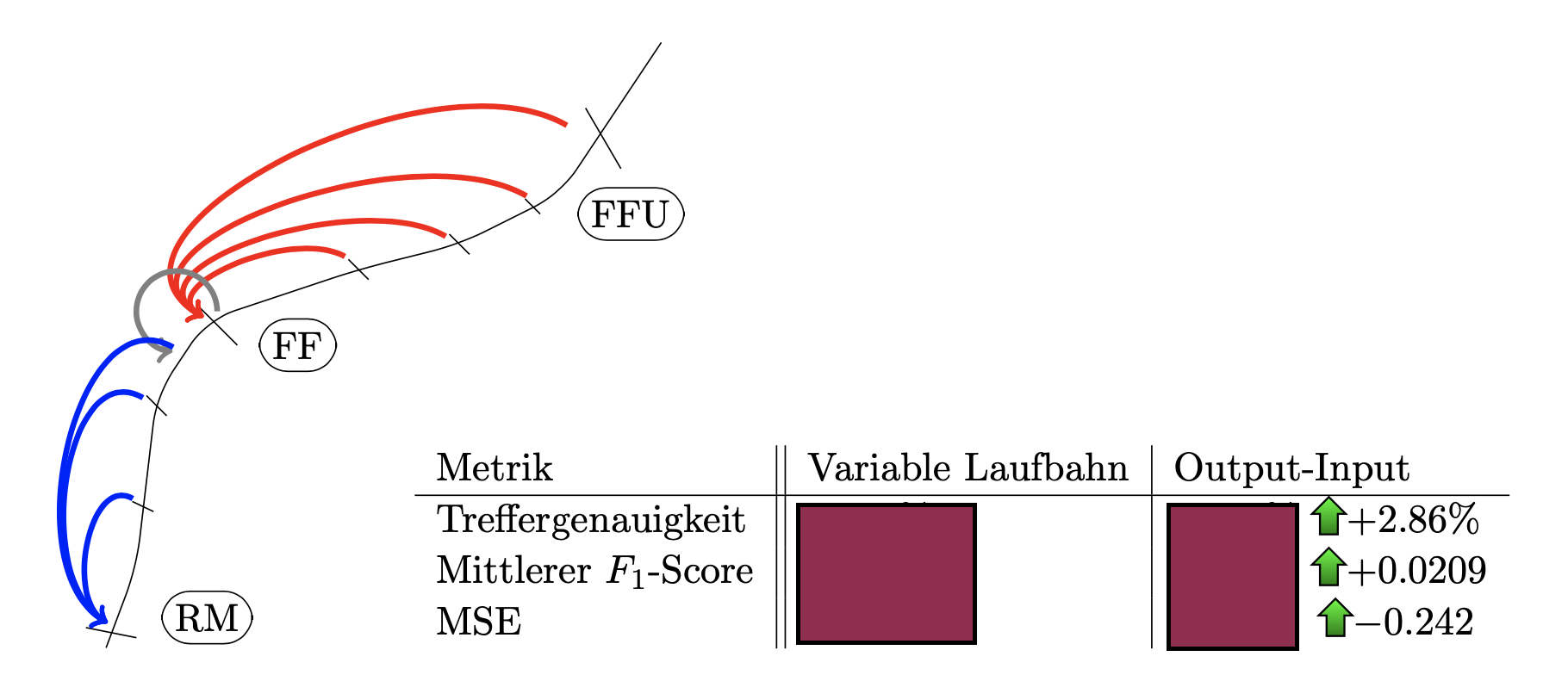 Fig: Approach 3: Output-Input.
Evaluation and Assessment: For the best result, we have used a regression problem with XGBoost regressor for every track section except the last one and a multiclassification with an XGBoost classifier for the last section.
We actually get better with the approach than the variable route approach. The results suggest that we were able to incorporate the dynamics of the track sections through our model. However, passing the output of one model into the next leads to error propagation. The error of one model is passed on to the next model. The next approach skips this step.
6.3.4. Approach 4: Segment by Segment
Here, as in the previous approach, we consider the route in sections. However, here we will make predictions directly for the endpoint and not for individual segments. Since the route segments and stops are now “constant” for each observation, we can also create specific features for route segments and stops for each observation. With this approach we create models for each segment.
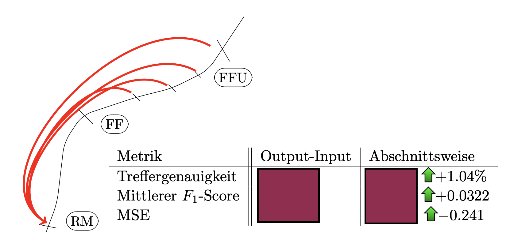 Fig: Approach 4: Segment by Segment.
Evaluation and Assessment: The best results are obtained by a multiclassification problem with XGBoost classifier. After a long search for the best approach, we found one that solves both problems: We get a lot of data from the approach and can capture the dynamics that exist on this route by classifying it in section-wise models. Compared to the relative position, our model is better in each selected metric.
In the next step we will further improve the results with stacking.
Stacking: The question of which base learner and meta learner to use is not an easy one. There are also no clear models in the literature that work better than others. It is small experimental steps that one has to take to find out what works for our problem and what does not. After much searching, we built a stacking model that trains 19 base learners with an XGBoost classifier as the meta learner.
 Fig: Segment by Segment with Stacking.
7. Conclusion and Outlook
By analyzing different solution approaches, we have recognized that the “section-by-section” solution approach delivers the best results. The performance can be increased with the ensemble method Stacking. The machine learning algorithms Random Forest, XGBoost, OneVsRest, Neural Networks, OrdinalClassifier and Logistic Regression were used and written in Python. For traditional Machine Learning algorithms we used the library sklearn and for Deep Learning algorithms keras, based on Tensorflow.
We narrowed our analysis in 3 ways: Time period, train type and track. By extending the time period (data available up to 2014), we can obtain more training data and thus increase the performance of the model if necessary, since machine learning algorithms generally perform better when they have more data. We obviously want to be able to use delay prediction on other rail lines. It would be interesting when analyzing on other corridors to see if the approach performs well on other routes as well, or if in some way we have overfitted the approach to the selected route. The same reasoning applies to an analysis for different train types.