In this post, I will summarize my Bachelor Thesis (Full Title: Nonparametric Regression Using Deep Neural Networks with ReLU Activation Function). Please find the comprehensive version here (unfortunately only in german). Find a presentation of this thesis here.

Table of Contents

1. Introduction and Motivation
   1. Goal of this Thesis
   2. Nonparametric Regression
      1. Parametric vs. Nonparametric Regression
   3. Convergence Rate
2. Description of the model
   1. Hierarchical composition of the regression function
3. Main Result
   1. Upper bound Of the L2 Error
      1. Conclusions from Theorem 1
   2. Lower Bound of $L_2$ Error
   3. Proof of Upper and Lower Bounds
4. Examples
   1. Additive Models
   2. General Additive Models
5. Conclusion

1. Introduction and Motivation

This work is based on the scientific paper Nonparametric regression using deep neural networks with ReLU activation function by Johannes Schmidt-Hieber, cf. , and deals with the topic of Deep Learning, one of the most discussed topics in statistics today. The interest is due to the development of the technology and the digitization. These two factors have made it possible to effectively use deep neural networks, the tools of deep learning, to be used effectively. Indeed, neural networks require not only powerful computers, but also a very large amount of data. Only digitization has made it possible to collect personal data, digital photos, sensor data and more, through powerful memory cards, social media platforms, smartphones and precise sensors. In contrast, traditional Machine Learning algorithms do not effectively exploit this amount of data.

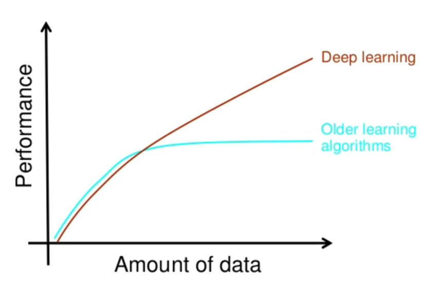
Over the past few years, deep learning methods have produced impressive practical results, such as the Object recognition in images. In this process, so-called convolutional neural networks process images as input to identify specific objects in the image. However, the application in image processing is only one of many areas in which neural networks are already the State-of-the-Art. However, the technology has developed faster than the theory, which raises the question of how the observed phenomena in practice can be explained in a statistical manner.

In the 1st chapter “Introduction and Motivation” introduces important terms, which are essential for the understanding of the thesis. In the 2. Chapter “Description of the Model”, we will define our neural network and define the framework of the model. In the section we will also define the considered network class and Function class of the regression function. The main theorems and proofs can be found in the 3rd chapter main results. Under the 4th chapter we discuss the additive and generalized additive models as examples. In the last chapter we will mention the main results of this work and discuss improvements and extensions of the model.

1.1. Goal of this Thesis

In this paper, we consider a multivariate nonparametric regression model and assume that the regression function consists of a composition of functions. The goal of this work is to find and prove an upper bound for the $L_2$-error, assuming that the deep neural network is sparsely connected with ReLU activation functions. From the results we can conclude that under certain conditions, deep feedforward neural networks avoid the curse of dimensionality. We will subsequently develop a lower bound for the $L_2$-error. Under the same assumptions, we can use it to calculate the minimax convergence rate for estimators from such networks (except for one that is logarithmic in sample size $n$ logarithmic factor). The results in this thesis will also show, among other things, that the depth of a neural network should increase with the number of training data to obtain the best results. Before doing so, however, we need to introduce some terminology which are essential for the understanding of this work.

1.2. Nonparametric Regression

We will first define the statistical problem that we treat in this paper. In the regression analysis we consider a random vector $(\mathbf{X},Y)$ with values in $\mathbb{R}^d \times \mathbb{R}$, where $E( Y^2 ) < \infty$. The goal of the analysis is to find the value for $Y$ from the observation vector $\mathbf{X}$ to predict. Mathematically, this relationship can be represented as

The noise variable is a standard normally distributed random variable that is is independent of $\mathbf{X}$. The goal now is to find a (measurable) function $f’: \mathbb{R}^d \to \mathbb{R}$ such that. $f’(\mathbf{X})$ approximates our $Y$ as well as possible. A so-called loss function is a measurable function $L: \mathbb{R} \times \mathbb{R} \rightarrow \mathbb{R}_{\geq 0}$, which gives us a measure of how well we have approximated $Y$ with our function. A so-called loss function is a measurable function $L: \mathbb{R} \times \mathbb{R} \rightarrow \mathbb{R}_{\geq 0}$ which gives us a measure of how well we have approximated $Y$ with our function. However, since $\mathbf{X},Y$ are now random variables, we cannot simply minimize $\vert L(Y,f’(\mathbf{X})) \vert$ since this is itself a random variable, but we minimize $E[L(Y,f’ (\mathbf{X}))]$, also called the risk.

One choice for the loss function, which we will motivate in Section 3, is the squared loss function $L(y,s) = (y-s) ^2$. It follows for the risk $E[L(Y,f’(\mathbf{X})] = E (\vert Y-f’(\mathbf{X})\vert^2)$, which is also called the mean squared deviation of $f’$ or $L_2$- risk. We thus look for a function $f_0: \mathbb{R}^d \rightarrow \mathbb{R} $ that minimizes the mean square deviation, i.e. $f_0$ should fulfill

To find out what exactly $f_0$ looks like now, we define $m:\mathbb{R}^d \to \mathbb{R},\ m = E (Y \vert \mathbf{X} = \mathbf{x})$ and consider an arbitrary function $f’: \mathbb{R}^d \to \mathbb{R}$ with the equation

where we take these as given and will not derive them in this thesis.

It is easy to see that $m$ is our sought function, because $E (\vert f’(\mathbf{X})-Y\vert^2)$ becomes minimal exactly when $f’ = m$. We call the function $f_0 = m = E (Y \vert \mathbf{X} = \mathbf{x})$ regression function.
The expression $E (\vert f’(\mathbf{X})-m(\mathbf{X})\vert^2)$ is also called $L_2$-error of $f’$. Thus, we can represent the $L_2$ risk as a sum of the $L_2$ risk of the regression function, also called the unavoidable error, and the $L_2$ error of $f’$.

However, there is a hidden problem: we do not know the distribution of $(\mathbf{X},Y)$, so estimating $Y$ by the regression function $ f_0 = E (Y \vert \mathbf{X} = \mathbf{x})$ is not possible. But if we are given data that is subject to the same distribution as $(\mathbf{X},Y)$, we have the ability to estimate $f_0$ through the data. The statistical problem is now to find a function $f_n: \mathbb{R}^d \to \mathbb{R}$ to estimate the regression function $f_0$ by given observations $D_n = {(\mathbf{X}_1, Y_1, … , \mathbf{X}_n,Y_n)}$ to be constructed, where $(\mathbf {X},Y), (\mathbf{X}_1, Y_ 1), …, (\mathbf{X}_n,Y_n)$ are u.i.v. random variables. It holds that the function $f_n (\mathbf{x}) = f_n(\mathbf{x},D_n)$ is measurable with respect to $\mathbf{x}$ and the data. The goal now, given the data $D_n$, is to construct a function $f_n(\cdot) = f_n(\cdot, D_n)$ such that its $L_2$ errors $E (\vert f_n (\mathbf{X})-f_0(\mathbf{X})\vert^2)$ are minimal.

1.2.1. Parametric vs. Nonparametric Regression

Next, let us explain the difference between parametric and nonparametric regression. In parametric regression, it is assumed that the structure of the regression function is known and, in addition, it is assumed that it depends only on finitely many parameters, but their values are unknown. These unknown values will now be estimated from the data. For example, in linear regression, the regression function is assumed to be linear and we estimate, the finite number of factors of the linear combination. However, there are significant drawbacks to parametric regression because we must first extract a structure from the data, which is often not immediately apparent.

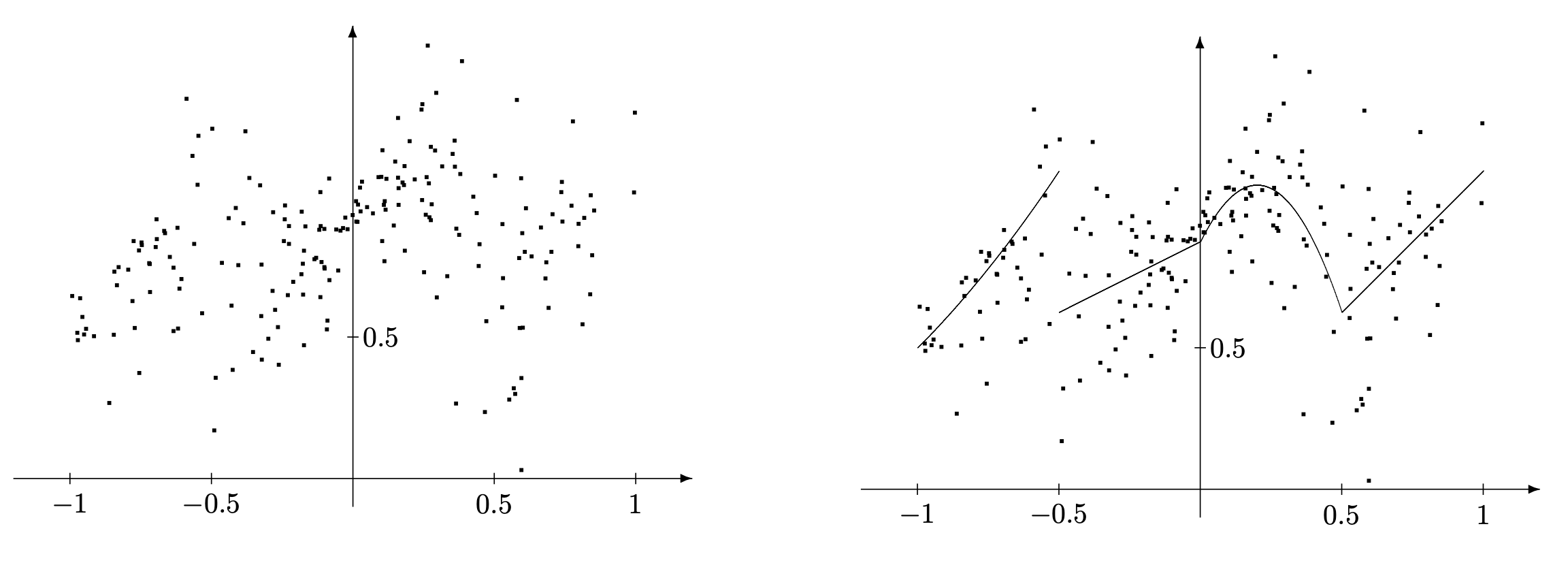The regression function cannot be directly assumed to have structure with the naked eye. In addition, if the assumed structural assumption is violated, bad estimates can arise very quickly.

In contrast, nonparametric regression assumes that the regression function does not have a functional structure that can be described by finitely many parameters. Only certain general regularity conditions are imposed, such as continuity, differentiability, or Hölder continuity. Thus, we can make a more general structural assumption on the regression function. Here, the regression function is estimated from the data, and there are several methods, such as neural networks, kernel regression, and KNN estimators.

1.3. Convergence Rate

In this paper, we will focus on neural networks and their possible advantages over other estimators. Primarily, we will analyze the advantage arising from the convergence rate.

To measure the error of an estimator $f_n$ of a regression function $f_0$, we use the $L_2$ error, as motivated above, and define it as

where $P_X$ is the distribution of the random variable $\mathbf{X}$. The estimator $f_n$ depends on the data $D_n$.
Of course, one wants to find an estimator for which the $L_2$ converges to 0 (with the number of observations) as fast as possible. We still have not constrained the distribution $(\mathbf{X},Y)$ in any way except that $E(Y^2) < \infty $ must hold. Unfortunately, there is no estimator for which the $L_2$ error converges to 0 for all distributions of $(\mathbf{X},Y)$ with a fixed rate of convergence, i.e., for any estimator the rate of convergence can be arbitrarily slow.

Thus, we need to restrict our distribution class in which the distribution of $(\mathbf{X},Y)$ lies in order to obtain nontrivial convergence rates. However, before we can analyze the optimal convergence rate of an estimator given a distribution class, we must first define what optimal means in this context. We speak of an optimal convergence rate if the rate is equal to the minimax convergence rate. Thus, we need to introduce the minimax convergence rate.

For a given class $D$ of distributions of $(\mathbf{X},Y)$, we try to find the maximum $L_2$ error within class

by an estimator $f_n$, i.e., the estimator should be close to the value of

lie, where we minimize over all regression estimators here. Since we are interested in the asymptotic behavior, we introduce the following terms:

Definition 1. A sequence of positive numbers $(a_n)_{n \in \mathbb{N}}$ for the class $D$ of distributions $ (\mathbf{X},Y)$ is called

• a) lower minimax convergence rate for D $\Leftrightarrow$

• b) upper minimax convergence rate for D if $f_n$ holds for an estimation method

• c) optimal minimax convergence rate for D if $(a_n)_{n \in \mathbb{N}}$ is lower and upper minimax convergence rate for D.

We had already said that we need to restrict the distribution class of $(\mathbf{X},Y)$ to get nontrivial solutions, so we make a typical assumption of nonparametric statistics. We assume that the regression function $\beta$ is smooth.

Stone had determined for $\beta$-smooth regression functions that the optimal convergence rate is $n^{-\frac{2\beta}{2\beta+d}}$, where $d$ is the dimension of the input. However, neural networks often deal with problems with high-dimensional input, which is why the optimal convergence rate is large, i.e., the convergence rate for such problems is very slow. Any statistical method would thus perform poorly, including our neural network. To understand how much this phenomenon limits our model, let’s do a small numerical example. Let be given a sample size of $n=100$, input dimension $d=100$ and smoothness $\beta = 2$. If the input dimension increases to $d=1036$, then to get the same convergence rate, you would have to have a sample size of $n = 500^{10}$! Even in today’s world, this amount of data is practically impossible.

However, it has been shown that neural networks do not suffer from the so-called curse of dimensionality . In this paper, we will investigate, among other things, under which conditions and how exactly neural networks avoid the curse by analyzing the convergence rate of the $L_2$ error.

2. Description of the model

Please see the full thesis for a comprehensive description of the model. In this post, we will only introduce essential parts of the model.

2.1. Hierarchical composition of the regression function

We assume a $\beta$-smooth regression function $f_0: [0,1]^d \rightarrow \mathbb{R}$. By rescaling the interval $[0,1]^d$, all results shown can be applied to any compact set $\mathbf{X} \subset \mathbb{R}^d$.
However, a minimax convergence rate of $n^{-2 \beta / 2\beta + d}$ for the $L_2$ error holds for $\beta$-smooth function, as we have already seen in Section 1.3. where $d$ is the dimension of the input. In Section 1.3. we have already motivated that we cannot achieve fast convergence rates under these assumptions.

In practice, however, we observe something different: neural networks seem to avoid the curse of dimensionality. The previous, very general model assumption thus seems implausible. Thus, the function classes we want to estimate must be much smaller than assumed.

Additional structural assumptions must be made on the regression function that allow us to achieve faster convergence rates, thus explaining the results of practice. The assumptions here should hold for problems where neural networks actually show better results. A heuristic idea is that neural networks perform well on problems where it is possible to build complex objects by simple objects in an iterative way. Such a structure is also called hierarchical structure. This idea can be heuristically reasoned from physics, mathematics and from neuroscience.

Mathematically, we can formulate this hierarchical structure as a regression function $f_0$ consisting of a composition of functions, i.e.

with $g_i:[a_i, b_i]^{d_i} \rightarrow [a_{i+1}, b_{i+1}]^{d_{i+1}}$, where $[a_i, b_i]$ is an interval. We denote the individual components of $g_i$ by $g_i = (g_{ij})_{j=1,…,d_{i+1}}^T$ and $t_i$ as the maximum number of variables on which each $g_{ij}$ depends. The $g_{ij}$ are thus $t_i$-variate functors. A simple example would be a bivariate function $f(x,y)$ that depends on only 2 variables. Of course, $t_i \leq d_i$ must always hold. The lack of uniqueness of the representation does not hurt us, since we are not interested in what exactly $g_0, …,g_q$ and the pairs $(\beta _i, t_i$) look like, but we will just exploit the property that $f_0$ consists of compositions of functions to ultimately estimate $f_0$.

To understand how each dimension interacts, let’s look at the following example to determine $d_i$ and $t_i$:

The maximum number of variables on which $g_{01}$ and $g_{02}$ depend are $t_{01} =1$ and $t_{02}=1$. It follows that $t_0=1$ holds.

In our $d$-variate regression model $f_0: [0,1]^d \rightarrow \mathbb{R}$ obviously $d_0 = d, \ a_0 = 0, \ b_0= 1, \text{ and } d_{q+1} = 1. $ Obviously, there are several ways to write the regression function in a composition, however, among all the ways to represent $f_0$, one should always choose one that gives the fastest rate of convergence.

One of the classical approaches of nonparametric statistics is to assume that the functions $g_{ij}$ are in the Hölder class with smoothness index $\beta_i$ . The definition of the Hölder class with smoothness index $\beta$ is:

Definition 2. Let $ \beta = q + s$ for a $q \in \mathbb{N}_0$ and $ 0 < s \le 1 $. A function $f: \mathbb{R} ^d \to \mathbb{R}$ is in the Hölder class with smoothness index $\beta $, if for each $\boldsymbol{\alpha} = (\alpha_1, …, \alpha_d) \in \mathbb{N}_0 ^d$ with $\sum \limits_{j = 1}^{d} \alpha_j = q $ the partial derivative $\vert{ \frac{\partial ^q m}{\partial x_1 ^{\alpha _1}…\partial x_d ^{\alpha _d}}(\mathbf{x}) - \frac {\partial ^q m}{\partial x_1 ^{\alpha _1}…\partial x_d ^{\alpha _d}}(\mathbf{z}) }\vert \le C \cdot \Vert \mathbf{x}- \mathbf{z} \Vert ^s$ for all $\mathbf{x},\mathbf{z} \in \mathbb{R} ^d$, whereas $\Vert \cdot \Vert$ is the euclidean norm.

Thus, a function is in the Hölder class with smoothness index $\beta $ if all partial derivatives up to degree $\lfloor \beta \rfloor$ exist, are bounded and the partial derivatives with degree $\lfloor \beta \rfloor$ are $\beta - \lfloor \beta \rfloor$ Hölder continuous, where $\lfloor \beta \rfloor$ is the largest integer strictly smaller than $\beta$. The ball of $\beta$-Hölder functions with radius $K$ is defined as

where $\partial ^{\boldsymbol{\alpha}} = \partial ^{\alpha _1}…\partial ^{\alpha _r}$ a multi-index with $\boldsymbol{\alpha} = ( \alpha _1, …, \alpha _r) \in \mathbb{N}^r$ and $\vert \boldsymbol{\alpha} \vert := \vert \boldsymbol{\alpha} \vert _1$.

3. Main Result

As a reminder, we study a $d$-variate nonparametric regression model whose regression function $f_0$ is in the class $G(q,\mathbf{d}, \mathbf{t}, \boldsymbol{\beta}, K)$. Here we consider an estimator $\widehat{f}_n$, which comes from the network class $F(L,\mathbf{p},s, F)$. Our goal is to find the minimax convergence rate for the $L_2$ error $R(\widehat{f}_n,f_0) = E _{f_0}[(\widehat{f} _n (\mathbf{X}) - f_0 (\mathbf{X}))^2]$ with $\mathbf{X} \overset{D}{=} \mathbf{X_1}$ independently of a given sample $(\mathbf{X}_i, Y_i)_i$. The index $f_0$ in $E _{f_0}$ denotes here the observation of the expected value, related to a generated sample from the model of nonparametric regression with the regression function $f_0$.

We will first give an upper bound in the 3.1. section for the $L_2$-error for estimators from the network class $F(L,\mathbf{p},s, F)$. In the section 3.1.1. we will list upper bound corollaries, such as bypassing the curse of dimensionality. In section 3.2. we will give a lower bound for the $L_2$-error. If these two bounds are identical, we can infer the minimax convergence rate. However, we will see later that our bounds differ by a factor of $L \log^2(n)$, so we still lack precision.

3.1. Upper bound Of the L2 Error

Theorem 1. Consider the $d$-variate nonparametric regression model for composite regression function in the class $(q,\mathbf{d}, \mathbf{t}, \boldsymbol{\beta}, K)$. Let $\widehat{f} _n$ be an estimator taking values in the network class $F(L, (p_i)_{i = 0,…, L+1}, s, F)$ satisfying

• The neural networks used for estimation allow function values at least as large as the maximum function values of the regression function $f_0$: $F \geq \max(K,1)$
• For the number of layers, let $\sum\nolimits_{i=0}^q \log _2(4t_i \vee 4 \beta _i) \log _2 n\leq L \lesssim n \phi _n$
• The size of the layers must go to infinity at least with rate $n\phi_n$ in $n$: $n \phi _n \lesssim \min _{i = 1,… ,L} p_i$
• Number of non-vanishing entries of weight matrices and displacement vectors must go to infinity with rate $n \phi_n \log(n)$ in $n$: $s \asymp n \phi _n \log n$

Then there exist constants C and C’ which depend only on q, d, t, $\boldsymbol{\beta}, F$, so that if $\Delta _n(\widehat{f}_n, f_0) \leq C \phi _n L \log ^2(n)$ holds, then

and if $\Delta _n (\widehat{f_n}, f_0) \geq C \phi _n L \log ^2 (n)$, then

The best choice for $L$ to minimize the rate $\phi _n L \log^2(n)$ is to choose $L$ proportional to $\log_2 (n)$. Thus, the number of layers should approach infinity with rate $\log_2(n)$ in $n$, i.e., $L \asymp \log_2(n)$. It follows $\Delta _n(\widehat{f}_n, f_0) \leq C \phi _n \log^3(n)$ and thus also

There is a tradeoff in the convergence rate $\phi_n$: If $t_i$ is large, this can be compensated by correspondingly large $\beta^*_i$.

3.1.1. Conclusions from Theorem 1

It follows from Theorem 1 that the convergence rate of the $L_2$-error, under the same assumptions, depends on $\phi_n$ and $ \Delta _n(\widehat{f}_n, f_0)$. From the following section 3.2. we can see that $\phi_n$ is the lower bound of the minimax of the $L_2$ error over the same class of functions, as from Theorem 1. From $\phi_n := max_{i=0,…q} n^{- \frac{2 \beta_i^*}{2 \beta_i^* + t_i}}$ we can see that the rate no longer depends on the original input dimension $d$, but on the $t_i$, which can be much smaller than $d$ if necessary. The $t_i$ can thus also be seen as the effective dimension that allow faster convergence rates to be achieved. Due to this, the network avoids the curse of dimensionality for certain structures of $f_0$.In addition, $\Delta _n(\widehat {f}_n, f_0)$ occurs in the lower bound and is thus unavoidable in the convergence rate. The expression $\Delta _n(\widehat{f}_n, f_0)$ takes a large value if $\widehat{f}_n$ has a large empirical risk compared to the minimizer of the empirical risk.

However, if $\widehat{f}_n$ is a minimizer of empirical risk, $\Delta_n = 0$ holds by definition. The condition $\Delta _n(\widehat{f}_n, f_0) \leq C \phi _n L \log ^2(n)$ from Theorem 1 is now trivially satisfied in this case, since $\Delta _n(\widehat{f}_n, f_0) = 0 \leq C \phi _n L \log ^2(n)$. Corollary 1 follows.

Corollary 1. Let $\widetilde{f}_n \in argmin_{f \in F(L,\mathbf{p},s,F)} \sum_{i=1}^n(Y_i-f(\mathbf{X}_i))^2 $ the minimizer of empirical risk. Under the same conditions as in the theorem 1, there exists a constant $C’$ that depends only on $q, \mathbf{d}, \mathbf{t}, \boldsymbol{\beta}, F $, so that

Thus, if we find a minimizer of the empirical risk, we would have an upper bound on the $L_2$ error of $\phi _n L \log^2(n)$. Unfortunately, the methods we use today, such as stochastic gradient methods, do not reliably find the minimizer. Thus, it would be of great interest to learn a method to constantly find a minimizer of the empirical risk to circumvent the term $\Delta_n$ in the convergence rate. Next, let us take a closer look at the conditions of Theorem 1.

Condition (i) from Theorem 1 is a very mild condition on the network function, since it only states that the function should have at least the same supremum norm as the regression function.

From condition $(ii$), we see that finding an upper bound on $t_i\le d_i$ and smoothness index $\beta_i$ is sufficient for choosing the network depth $L$. We have already seen that the best choice for the number of hidden layers is $L \asymp \log_2(n)$. Thus, the depth of the neural network should grow with the sample size.

The network width $\mathbf{p}$, which is constrained in condition $(iii)$, can be chosen independently of the smoothness indices by satisfying $n \phi _n \lesssim \min _{i = 1,…,L} p_i$ instead of $n \lesssim \min _{i = 1,… ,L} p_i$. Namely, $\phi_n \leq 1$ holds and thus $n \phi _n \lesssim n \lesssim \min _{i = 1,…,L} p_i$ follows if $n \lesssim \min _{i = 1,…,L} p_i$ holds. For example, one could choose the sample size $n$ as the width for each hidden layer.

From the condition (iv) we can conclude that we must have a sparse network must be present. The reason is that in a fully connected network the number of weight parameters $\sum_{i=0}^L p_i p_{i+1}$ and for the displacement parameters $\sum_{l=1}^{L} p_L$. Thus, the magnitude of the network parameters is $\sum_{i=0} ^L p_i p_{i+1}$. However, it holds

and with the conditions (iii), (ii) it follows

and thus the condition (iv) cannot be satisfied. This shows that Theorem 1 assumes $sparse$ networks. In fact, it holds that the network must have at least $\sum _{i=1}^L p_i - s$ inactive nodes, that is, all incoming ones of these nodes are zero. The statement can be justified by the following consideration: With a fixed number of active network parameters $s$, we achieve the highest number of active nodes by including no active displacement parameters but only active weight parameters in the network. Thus, we have $s$ active weight parameters. Now, to generate as many active nodes as possible, we only connect to inactive nodes until we have no weight parameters or no inactive nodes left. This obviously achieves at most $s$ active nodes in the hidden layers. It follows that there are at least $\sum _{i=1}^L p_i - s$ inactive nodes.

The choice $s \asymp n \phi _n \log (n)$ in condition $(iv)$ balances the squared bias and variance. From the proof of Theorem 1, one can see that the rate of convergence can also be derived for other orders of magnitude of $s$.

From the conditions in Theorem 1 we can deduce that we have a very flexible way to choose a good network architecture as long as the number of active parameters $s$ satisfies condition $(iv)$. Thus, the size of the network does not play the most important role for the statistical performance, but the proper regulation of the network with respect to the number of active parameters from condition $(iv)$!

3.2. Lower Bound of $L_2$ Error

Theorem 2. Consider a d-variate nonparametric regression model with observations $\mathbf{X}_i$ from a probability distribution with a Lebesque density on $[0,1]^d$, which is constrained with an upper and lower positive constant. For any non-negative integer q, any dimension vectors d and t satisfying $t_i \leq \min (d_0,…, d_{i-1})$ for all i, any smoothness vector $\boldsymbol{\beta}$, and any sufficiently large constant $K > 0$, there exists a positive constant c such that

where the $\inf$ is taken over all estimators $\widehat{f}_n$.

We see by Theorem 2 that $\phi_n$ is a lower bound for the minimax $L_2$-error over the function class $G(q,\mathbf {d},\mathbf{t}, \boldsymbol{\beta}, K)$. Recall that the theorem 1 gives us an upper bound on the $L_2$ error for an estimator from the network class $F(L,\mathbf{p},s, F)$ over the class $G(q,\mathbf{d},\mathbf{t}, \boldsymbol{\beta}, K)$. Now, if both bounds were to match, we could infer from the two (identical) bounds that estimators from sparse deep neural networks achieve the minimax convergence rate. However, since we have a lower bound for the $L_2$ error with $\phi_n$ on the one hand and an upper bound for estimators from $F(L,\mathbf{p},s, F) $ with $\phi_n L \log^2(n)$ on the other hand, with which our bounds do not coincide, we still have a gap in our theory here. Thus it could be that our lower bound from Theorem 2} or our upper bound from Theorem 1 are too inaccurate. Johannes Schmidt-Hieber conjectures that the factor $L \log^2(n)$ from the upper bound from Theorem 1 is an artifact from the proof. We can give a minimax convergence rate from Theorem 1 and 2 that differs up to $L\log^2(n)$.

3.3. Proof of Upper and Lower Bounds

To see the full proof, please see the thesis.

4. Examples

In this section we will look at models that formulate a stronger structural decomposition of the regression function $f_0$ than we did in Section 2. Thus, these are special cases.

4.1. Additive Models

In additive models, the regression function $f_0(\mathbf{x})$ is assumed to decay into a sum whose summands depend on only one component of $\mathbf{x}$.

Definition 2. Let $K > 0$. Let $f_0(\mathbf{x}) = \sum_{j=1}^d g_{0j} (x_j)$ with continuously differentiable functions $g_{0j}: \mathbb{R} \rightarrow [-K,K].$ Then it holds

whereas

The individual components of $g_0$ are differentiable only once, but have also only the definition range $\mathbb{R} $. On the other hand $g_1$ has the domain $\mathbb{R}^d$, but as a sum function it is infinitely differentiable.

Since the functions $g_{0j}$, $j=1,…,d$ are continuously differentiable with the range of values $[-K,K]$, for $g_0: [0,1]^d \rightarrow [-K,K]^d$ holds. Thus, we choose $g_1: [-K,K]^d \rightarrow [-Kd, Kd]$. The dimensions of the model are thus $d_0 = d$, $d_1=d$, $d_2 = 1$. The individual components of $g_0$ are continuously differentiable and depend on only one component at a time, so the effective dimension is $t_0= 1$ and the smoothness is $\beta_0 = 1$. The function $g_1$ is infinitely differentiable and consists of a sum of $d$ terms. Thus, it holds for the effective dimension $t_1 = d$ and $\beta_1 > 1$ arbitrarily large. In summary, we can say that the regression function is in the class $G(1,(d,d,1), (1,d), (1,\beta_1), (K+1)d)$.

The effective smoothness index is $\beta^*_0 = 1 \cdot (\beta_1 \wedge 1) = 1$ and $\beta^*_1 > 1$ can be chosen arbitrarily large. Next, we will calculate the convergence rate:

It follows with the effective smoothness indices

and thus follows for the convergence rate $\phi_n = n^{-2/3}$. If now the conditions

• (i) $F \geq (K+1)d$
• (ii) $L$ proportional to $\log_2(n)$: $\log_2(n)\left( \log_2(4)+\log_2(4d \vee 4 \beta_1) \right) \leq L \lesssim \log_2(n)$}
• (iii) $n^{1/3} \lesssim \min_i p_i$
• (iv) $s \asymp n^{1/3}\log(n)$

are satisfied by a network architecture $F(L,\mathbf{p},s,F)$, then we can convert the 2 distinct cases in the theorem 1 for the network to

4.2. General Additive Models

We assume that the regression function is of the form

where $h: \mathbb{R} \rightarrow \mathbb{R}$ is an unknown function. We can write the regression function as a composition $f_0 = g_2 \circ g_1 \circ g_0$ with $g_0$, $g_1$ as defined in the 4.1. section, and $g_2 = h$. We will assume this time that we have a more general form for the $g_{0j} \in C_1^\beta([0,1],K), \ j = 1,…,d$. Now let $h \in C_1^\gamma(\mathbb{R},K)$, then $f_0: [0,1]^d \overset{g_0}{\rightarrow}[-K,K]^d \overset{g_1}{\rightarrow} [-Kd, Kd] \overset{g_2}{\rightarrow} [-K,K]$. For any $\beta_1 > 1$, $g_1 \in C_d^ {\beta_1}([-K,K]^d, (K+1)d)$ holds. As justified for the additive models, holds

For the effective smoothness indices:

We can now conclude for the convergence rate that

and therefore

For network architectures satisfying the conditions of Theorem 1, the following holds true

5. Conclusion

In this section, we will discuss the value of the work itself and the results presented here in the context of statistical elaboration of deep learning methods. Finally, we will address possible improvements and extensions to the model to further close the gap between theory and practical implementation.

Under a hierarchical structure of the regression function, the deep neural networks can adapt to the underlying structure in the signal and can thus avoid the curse of dimensionality. The results show for the first time that one can achieve (near) optimal convergence rate with sparse multilayer neural networks with ReLU activation function. For the proof, one uses new approximations for multilayer feedforward neural networks with constrained weights and constrained width of layers. While there has been previous statistical work, a much more general and real-world setting is now adopted than was done in earlier work. Important implications, under the same framework as in the main Theorem 1, are once that the hidden layers should grow with the sample sizes with $L \asymp \log_2(n)$ and that the network can have more parameters than the number of samples. Another important finding is that the most important factor for statistical performance is not the size of the network, but the regulation of the network, i.e., the number of active parameters. The results also give us an explanation why such networks work well in practice.

A major limitation is that we are considering a deep feedforward neural network. However, many of the latest deep learning applications are based on other specific networks, such as a convolutional neural network or recurrent neural network. So it is natural to ask how to statistically study such types of networks and analyze the convergence rate there as well.

An obvious improvement to the model would be to improve the inaccuracy we already mentioned in the 2. section in our lower and upper bounds, respectively. Heuristic results show that probably the factor $L \log(n)^2$ in the upper bound is an artifact of the proof.

Another topic that could be interesting for the results of this work is the research of stochastic gradient descent. Here one deals nowadays with, for example, the escape of saddle points or local minima. So statements could be made how much the term $\Delta_n(\widehat{f}_n, f_0)$ decreases in $n$ using stochastic gradient descent or even other methods. However, the analysis would strongly depend on the method used. An independent analysis could be done by analyzing
the loss landscape of deep networks, i.e. how saddle points, local and global minima of the loss function are arranged and how we can characterize them. We could, if necessary, obtain an upper bound on the term $\Delta_n (\widehat{f}_n,f_0)$ and consider it in the theorem 1. In fact, there are first heuristic results for fully connected networks which see a connection to spherical spin glasses, which have already been studied in detail. There, all local minima lie with a high probability in a band which is obviously bounded downward by the global minima. The width of the band depends on the width of the network and also gives us an upper bound on the term $\Delta_n ( \widehat{f}_n, f_0)$ for all methods converging to a local minima. If we can mathematically consolidate this heuristic result, then we could consider the dependence of the term $\Delta_n ( \widehat{f}_n, f_0) $ on the width vector $\textbf{p}$ in our convergence rate.

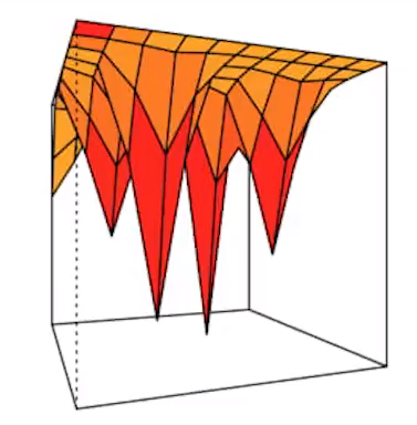Example loss landscape of a neural network.

We see that many questions that arise from the various areas of Deep Learning do not yet have a satisfactory answer. In a way, this work is intended to be a start to build statistical models that can be used to solve related problems, such as studying the convergence rate among other network types.

References

Full references in the thesis.

Schmidt-Hieber, Johannes: Nonparametric regression using deep neural networks with relu activation function. arXiv:1708.06633, März 2019.