
[Project] Cross-Lingual IR: Traditional vs. Modern
Published:
A project by Minh Duc Bui, Jakob Langenbahn, Niklas Sabel. Download the paper here. Download the presentation slides here.

Abstract
Cross-Lingual Information Retrieval is the task of getting information in a different language than the original query. Our goal is to implement a lightweight system, unsupervised and supervised, to recognize the translation of a sentence in a large collection of documents in a different language. Testing different cross-lingual word embeddingand text-based features with wide-ranging parameter combinations, our best model, the MLPClassifier, achieved a Mean Average Precision of 0.8459 on our EN-DE test collection. Our lightweight system also demonstrates zeroshot performance in other languages, such as Italian and Polish. We compare our results to the SOTA, but resource-hungry transformer model XLM-R.
1. Introduction
The rise of the Internet and the exponentially growing amount of multilingual data online makes it necessary for Retrieval systems to not only be able to query documents in the same language but in different languages as well.
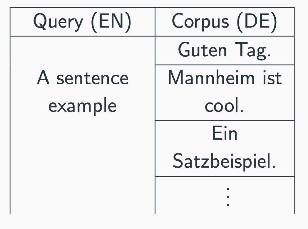 Task: Given a query in one language, recognize its translation from a large collection of sentences in another language.
Retrieving information in a different language requires the documents and the queries to be mapped into the same representation space. Since sparse representations based on machine translation face difficulties for resource-poor languages, dense representations derived via crosslingual word embeddings or multilingual text encoders like XLM-R became state of the art for Cross-Lingual tasks. These dense vectors can capture semantic associations between text representations far better in much smaller space leading to better results, especially when lower-resource languages are involved. However, as transformer models such as XLM-R are computational expensive to train, which lead to a large carbon footprint, the question remains if its size is necessary for tasks like translation retrieval.
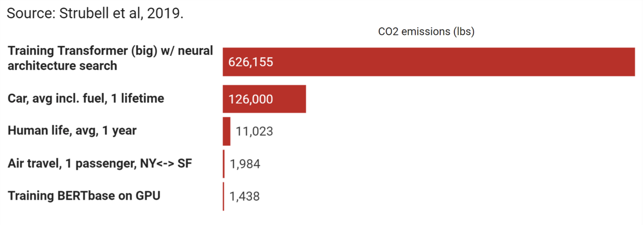
In this project, we want to answer a simple question: How far can we get with traditional, lightweight machine learning approaches and if the complexity of transformers justifies its means.
Our approach of creating a Cross-Lingual Information Retrieval system to get the translation of a query in a different language involves using different unsupervised methods and the training of traditional supervised methods based on cross-lingual word embeddings. We then contrast our approach to SOTA multilingual text encoders. Finally, to compare the models, we use the Mean Average Precision as our metric on the Europarl Corpus, a standard data collection for sentence-level CrossLingual Information Retrieval.
This report is divided as follows. In section 2 we describe our data and how we generated our feature vector to represent the information for our traditional supervised models. Then, in section 3, we show our implementation strategy for different supervised and unsupervised ranking methods and their performance on our task. To get a better estimation of the possibilities of our models, we evaluate them for different languages and on a document-level task in section 4. In section 5 we give a summary and discussion of our results.
2. Data
This section deals with the description of our data set and the preprocessing and the generation of the associated feature vector, which is later used to train our model. We distinguish between textbased features and embedding-based features created via different methods.
2.1. Europarl data set
Our project is based on data generated from the Europarl Corpus (Koehn, 2005). The corpus is extracted from proceedings of the European Parliament and can be easily accessed online. The corpus currently contains 21 different languages.
Our main section focuses on the parallel-corpus for German and English, containing 1,920,209 sentences with 44,548,491 words in German and 47,818,827 English words. In our evaluation, we also use our model on different language pairs, specifically English-Polish and EnglishItalian from the Europarl Corpus. The corpus for Polish and English contains 632,565 sentence pairs with 12,815,544 Polish and 15,268,824 English words. In comparison, the EnglishItalian corpus consists of 1,909,115 sentences with 47,402,927 Italian and 49,666,692 English words.
In the following, we focus on an extract of 220,000 sentence pairs from the EN-GER corpus, where 20,000 pairs represent correct translations and 200,000 pairs are wrong translations.
2.2. Sentence Generalisation
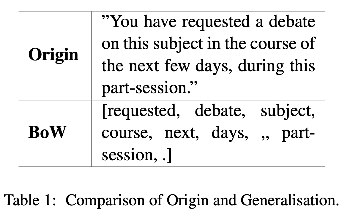
For our traditional supervised models, we first need to clean and generalize our aligned sentence pairs. Therefore, we tokenize both English and German sentences into bag-of-words representations to better handle individual words. Afterward, we lowercase all different words to prevent case sensitivity. At last, we remove all stopwords from our bag-of-words representations (BoW). Stopwords do not add much value to distinguish between different sentences, so we ignore them. We can see a comparison between our original sentence and the generalized sentence in Table 1 below. For the creation of embedding-based features, we additionally lemmatize all words and drop punctuation and numbers.
2.3. Induction of Multilingual Word Embedding Space
We study two approaches of inducing a multilingual word embedding: Projection-based CrossLingual Word Embeddings and pre-trained multilingual text encoders based on Neural Transformer architectures. Both methods are candidates for our supervised and unsupervised retrieval approach.
2.3.1. Projection-Based Models
Projection-based methods rely on independently trained monolingual word vector spaces in the source language $X_ {L1}$ and target language $X_{L2}$, that post-hoc align the monolingual spaces into one cross-lingual word embedding $X_{CL}$. The alignment is based on word translation pairs $D$, which can be obtained by existing dictionaries or by inducing it automatically. Applying existing dictionaries, we use bilingual supervision and, therefore, a supervised method. Inducing the embeddings automatically is an unsupervised approach and usually assumes (approximately) isomorphism between monolingual spaces.

We use Proc-B as a supervised method and VecMap as an unsupervised method. In both cases, we use the 300-dimensional fastText word vectors pre-trained on Wikipedia articles by (Bojanowski et al., 2016). We restrict the fastText vocabulary to the 100,000 most frequent terms in each language.
Proc-B (Supervised): Proc-B is a supervised projection-based method, so, we use a pre-obtained dictionary $D_w = (w_{L1}^k, w_{L2}^k)_{k=1}^{K}$ containing $K$ word pairs for finding the alignment, where $w_{L1}^k \in X_ {L1}$ and $ w_{L2}^k \in X_{L2}$ are translations of each other. We define the fastTest monolingual embedding spaces as $X_{L1}$ and $X_{L2}$ with the corresponding fastText vocabulary $V_{L1}$ and $V_{L2}$. Given the translation dictionary $D$, we can retrieve the corresponding monolingual vectors from $X_{L1}$ and $X_ {L2}$ and then construct aligned monolingual subspaces $X_S = (s^k_{L1})_{k=1}^K \subseteq X_{L1}$ and $X_T = (t^k_ {L2})_{k=1}^K \subseteq X_{L2}$, where the aligned rows are translations of each other. Mikolov et al. (2013) learns the projection $W_{L1}$, by minimizing the Euclidean distance between the linear projection of $X_S$ onto $X_T$:
\[W_{L1} = argmin \Vert X_{S} W X_{T} \Vert.\]To improve performance, we constrain $W_{L1}$ to be an orthogonal matrix (Xing et al., 2015). Then equation the previous equation becomes the Procrustes problem, which can be solved by a closed form solution, using the singular value decomposition of $X_S^T X_T$ (Schönemann, 1966):
\[\label{eq:2} \begin{split} W_{L1} & = U V^T ,\\ U \Sigma V^T & = \text{SVD}(X_S^T X_T). \end{split}\]Solving this equation corresponds to our method PROC. To further improve the quality of the linear mapping $W_{L1}$, which is restricted to the initial translation dictionary, we employ a bootstrapping approach to augment the initial dictionary, called PROC-B (Glavas et al., 2019).
To account for polysemy of words, we use the proposed train set of (Conneau et al., 2018) to align the monolingual word embeddings. The train set include different translations of the same word for each language pair consisting of the 5000 most frequent (unique) words in the source language and corresponding translation(s). Notice that the training set can contain more translation pairs than unique source words because each source word consists of multiple translation pairs. Furthermore, we only keep translation pairs, where the source and target word are contained in our (trimmed) fastText vocabulary.
For PROC, we use the full training set PROC($\sim$5k) and a smaller training set with 500 unique source words PROC($\sim$0.5k). Furthermore, we only use the bootstrapping technique for the smaller set PROC-B($\sim$0.5k) to improve performance as we did not notice any improvement (on BLI task) for the full training set.
VecMap (Unsupervised): VecMap (Artetxe et al., 2018) is a fully unsupervised method, which uses heuristics to build the seed dictionary. The method consists of 4 sequential steps:
- Normalize the embeddings by normalizing the length, centering the mean values of each dimension, and normalizing the length again.
- Unsupervised initialization of an initial solution (seed dictionary) assumes that the monolingual similarity distributions are approximately equal across languages.
- Robust self-learning procedure that iteratively improves the initial solution. VecMap uses different (empirically motivated) improvements for robustness, for example, stochastic dictionary induction, enabling the model to escape poor local optima.
- Final refinement of the final solution by symmetric re-weighting.
For more details, we refer to the original paper (Artetxe et al., 2018).
2.3.2. Pre-trained Multilingual Text Encoders
We use the implementation of a pretrained XLM-R (Conneau et al., 2020) from huggingface (Wolf et al., 2019), which is able to induce a multilingual, contextualized word embedding. Motivated by the results of Litschko et al. (2021), we exploit the contextualized representations by directly encoding the whole input text. To understand how we encode the text, let us assume that a term $t_i$ (i.e. a word-level token) is tokenized into a sequence of $K$ subword tokens. The model creates contextualized subword embeddings for each subword $\overrightarrow{wp_{i,k}}, \ k = 1,…, K$ of the term $t_i$. Following Litschko et al. (2021), we obtain the contextualized representation of each term $t_i$ by taking the representation of its first subword token:
\[\overrightarrow{t_i} = \overrightarrow{wp_{i, 1}}.\]To finally encode the whole input text, we compute the average of the contextualized representations of all terms $t_i$ in the text.
We use the embeddings from the first layer XLM-R(Layer 1) and the last layer XLM-R(Layer 12).
2.3.3. Evaluating on the BLI Task
In this section, we want to identify which induced cross-lingual word embeddings are useful for our supervised models to save computation later on. As we are going to use various distance measurements in the induced embedding to extract features for our downstream task (see Section 2.4.2), translations must be close to each other to extract meaningful features. For this purpose we evaluate on the BLI task.
 We test our multilingual word embeddings on the BLI task, using mean average precision (MAP) as metric. We take the proposed test sets of Conneau et al. (2018), which take the polysemy of words into account (1500 unique source words) and we average the MAP across 6 language pairs (EN-DE, EN-DU, EN-IT, ENPL, EN-FI and EN-RU).
Our intermediate results (Table 2) show that XLM-R and the low supervision variant of PROC are not suitable for extracting similarities, which is why we will not use them for our supervised method (and we want to avoid using the transformer model to be computational cheap). As PROC($\sim$0.5k), VecMap and PROC-B($\sim$0.5k) showed similar good results, we use all three to extract features for our supervised models, allowing our models to choose from a variety of different CLWE.
2.4. Feature Generation
We want to differentiate for two input sentences from different languages if they are direct translations of each other or not, denoted by $1$ if a sentence is a direct translation or $0$ otherwise. Therefore, we need to define a function $\psi$ that maps our input sentences into a vector $X_i=(x_{i1},…,x_{im}) $ consisting of $m$ features for each language pair that is used to train our model.
Therefore, we define two language spaces $L_1=\{l_{11},…,l_{1n}\}$ and $L_2=\{l_{21},…,l_{2n}\}$ describing the two languages respectively. Our input into $\psi$ is a tuple $(l_{1i},l_{2i})$ and a target label
\[y_i=\begin{cases} 1 & \text{right translation}, \\ 0 & \text{wrong translation}. \end{cases}\]So our function $\psi$ maps the original set $\{ (l_{1i}, l_{2i}), y_i) \}_ {i=1,…,n}$ to a training set $\{X_i,y_i\}_{i=1,…,n}$ via different preprocessing operations described in the following.
2.4.1. Text-Based Features
To begin with, we focus on features that are generated directly out of the bag-of-words representations using different techniques, including, e.g. counting of appearances. Then, we use different comparative figures as features, precisely absolute, relative, and normalized differences. When we derive these comparative features, we always use asymmetrical approaches to increase transferability for other translation tasks. So, we get the absolute
difference by subtracting the associated English amount from the German count and the relative difference by dividing the absolute difference with the sum of the English and the German count. Since it is clear that longer
sentences are more likely to have higher counts of, for example, words, we have to take into account that the length of sentences can vary a lot across different languages. Therefore, we also compute the normalized difference by first dividing the measure by the length of the sentence in the particular language. We now give an overview of all the text-based features that contribute to our model.
Number of (unique) words. Assuming that the number of words and especially unique appearances of words within a sentence has much impact on the meaning of a sentence, we count the number of words and the number of unique words separately for each of the sentences in both languages and compare them as described above.
Number of all punctuation marks. Under the hypothesis that punctuation marks have the same importance as the number of words, we count the number of all appearances as well as the amount of the following punctuation marks separately: Question marks, exclamation marks, commas, semicolons, colons, ellipsis, apostrophes, hyphens, quotation marks, slashes, brackets, and other special characters. The differences are calculated as described. We assume that especially the appearance of question and exclamation marks have a significant impact on our model performance since it is likely that two sentences are not a translation of each other if there is a difference between these two. However, we specifically excluded the amount of sentence-ending points and did not take them into account because we noticed that in some cases, two or more sentences in English are translated into only one German sentence and the other way around.
Number of characters. In addition, we include the number of characters per sentence. Further, we also take the average of characters per word because long sentences with many short words can have the same counts as short sentences with long words. However, it is unlikely that a sentence pair like that is a direct translation.
The following features are all based on POS-tagging with the already implemented spacy library, which allows us to handle NLP tasks for over 60 languages efficiently.
Number of word types. Based on our POS-tagging, we count the number of word types described by the core universal POS tag list, such as nouns, adjectives, or verbs, and only exclude punctuation marks from the list, as we already handled them. We get the absolute difference between the numbers across the different word types.
Verb times. Under the assumption that sentences are more likely to be direct translations if the verb times in both sentences match, we extract the different verb times with the help of the spacy package and compare the amount regarding past, present, and other verb times.
Jaccard coefficient of numbers. One feature is the Jaccard coefficient of the named number in the sentences in source and target languages. Given two sets, A and B, the Jaccard coefficient is calculated according to this formula:
\[Jaccard(A,B) = \frac{|A \cap B|}{|A \cup B|}\]2.4.2. Embedding-Based Features
Furthermore, we describe our approach to extract embedding-based features from our induced embedding space.
Jaccard coefficient of direct translations. The Jaccard coefficient of direct translations is calculated using the original sentence and its translation based on the cross-lingual word embedding. The word’s translation is the closest neighbor from the target language sentence corpus based on the distance of the cross-lingual word embeddings measured via cosine similarity. This is calculated for the translation from source to the target language and from target to source language. Both scores are then averaged to one single score.
Sentence Embedding Euclidean distance. We also derive the euclidean distance between the sentence embeddings from source and target. One sentence embedding aggregates the words by average, the other averages weighted by tf-idf.
Sentence Embedding Cosine Similarity. We also include the cosine similarity between the sentence embeddings from source and target and again aggregate by averaging or using tf-idf.
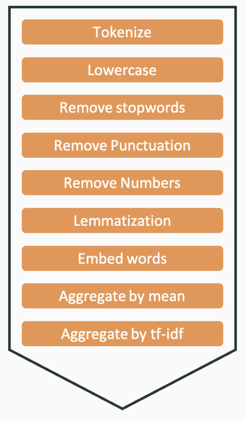 All possible steps of preprocessing.
3. Learning to Rank (L2R)
 High Level view of Unsupervised vs. Supervised Methods.
3.1. Unsupervised Ranking
First, we introduce an unsupervised ranking system to build a naive, but competitive baseline. We evaluate the cross-lingual word embeddings, produced by PROC(∼5k), PROC-B(∼1k) VecMap, XLM-R (Layer 1) and XLM-R(Layer 12), described in Section 2.3. To retrieve embeddings for the query q and all documents in the document collection D, we aggregate each word embedding by either averaging (AVG) or using tf-idf weighting (TFIDF). We use the cosine similarity (COS) as our similarity measure, and additionally, we use the Jaccard coefficient of direct translation (Jaccard) as another unsupervised ranking method. Finally, we rank the documents according to the measurements.
To choose the best unsupervised method, we evaluate on the validation set, described in Section 3.2.1. The results can be found in Table 3. First, we see that the multilingual embeddings, induced by the XLM-R model, lack quite far behind the other methods as they do not explicitly induce a cross-lingual word embedding, where word translations are near each other. All three projectionbased cross-lingual word embeddings behave similarly. The Jaccard coefficient of direct translations is significantly better than the cosine similarities. Looking into the ranking, we see that the cosine similarity sometimes rank sentences high that do not relate to the source sentence in any way. This shows that aggregating (averaging or tfidf) and then comparing word embeddings leads to higher false-positive rates. However, the Jaccard coefficient is much simpler and ”forces” a relation between source sentences and high-ranked sentences: Both should contain translations based on the cross-lingual word embedding.
As VecMap has the advantage of inducing the cross-lingual word embedding in an unsupervised fashion, which makes the ranking approach completely unsupervised and is not lacking far behind the best approach Proc(∼5k) with Jaccard, we choose VecMap with Jaccard to report on our test set.
3.2. Supervised Ranking
In the following section, we describe our approach to implement a supervised model that accurately detects the translation of a query sentence $q$ in a document collection $D$. Our result is a binary classification model that ranks the documents according to the confidence assigned to each of the different documents. We first describe our training, validation and test set used for judging and tuning our models. Afterward, we describe our different supervised models.
3.2.1. Train, Validation and Test Set
We aim to train a supervised classifier, and for that reason, we need to generate training, validation and a test set. As we already described, our training set is derived from our source and our target language via different preprocessing steps. Our final training set $X_{train} = \{ X_i,y_i \}_{ i=1 , … , n}$ contains $n = 220,000$ training examples , where each $X_i=(x_{i1},…,x_{im})\in \mathbb{R}^m$ represents our feature vector for a specific translation pair and $y_i$ is $1$ for relevant documents and $0$ for non-relevant documents. We retrieve the non-relevant documents by randomly subsampling 100 wrong translations (to reduce computation) and then calculating the cosine similarity between the given query $q$. We then take the five closest translations according to the cosine similarity measure in the cross-lingual word embedding induced by PROC($\sim$5k) as non-relevant documents.
Our classification model is described by a function $f:\mathbb{R}^m \to [0,1]$ that maps our feature vector to the confidence as translation score, with high scores more likely to represent a true translation.
Furthermore, we use a validation set to select features and tune the hyperparameter of the model. The validation set consists of a query-document collection derived from a set of queries $Q={q_1, …, q_s}$ and a set of documents $D={d_1, …, d_r}$ containing the right translation for each of the queries, where $s\ll r$. We create a query-document pair for each possible combination with the cartesian product of $Q$ and $D$. We generate the validation set by applying our preprocessing function $\psi$ to the cartesian product. We use our model to assign a translation score to each pair and rank them according to the score. We chose query collection of size $s = 100$ and a document collection of size $r = 5,000$. So, our whole validation set is of size $t = 500,000$. The independent test set is constructed in the same way as the validation set with the same sizes and it does not contain any sentence seen during training and feature/hyperparameter selection.
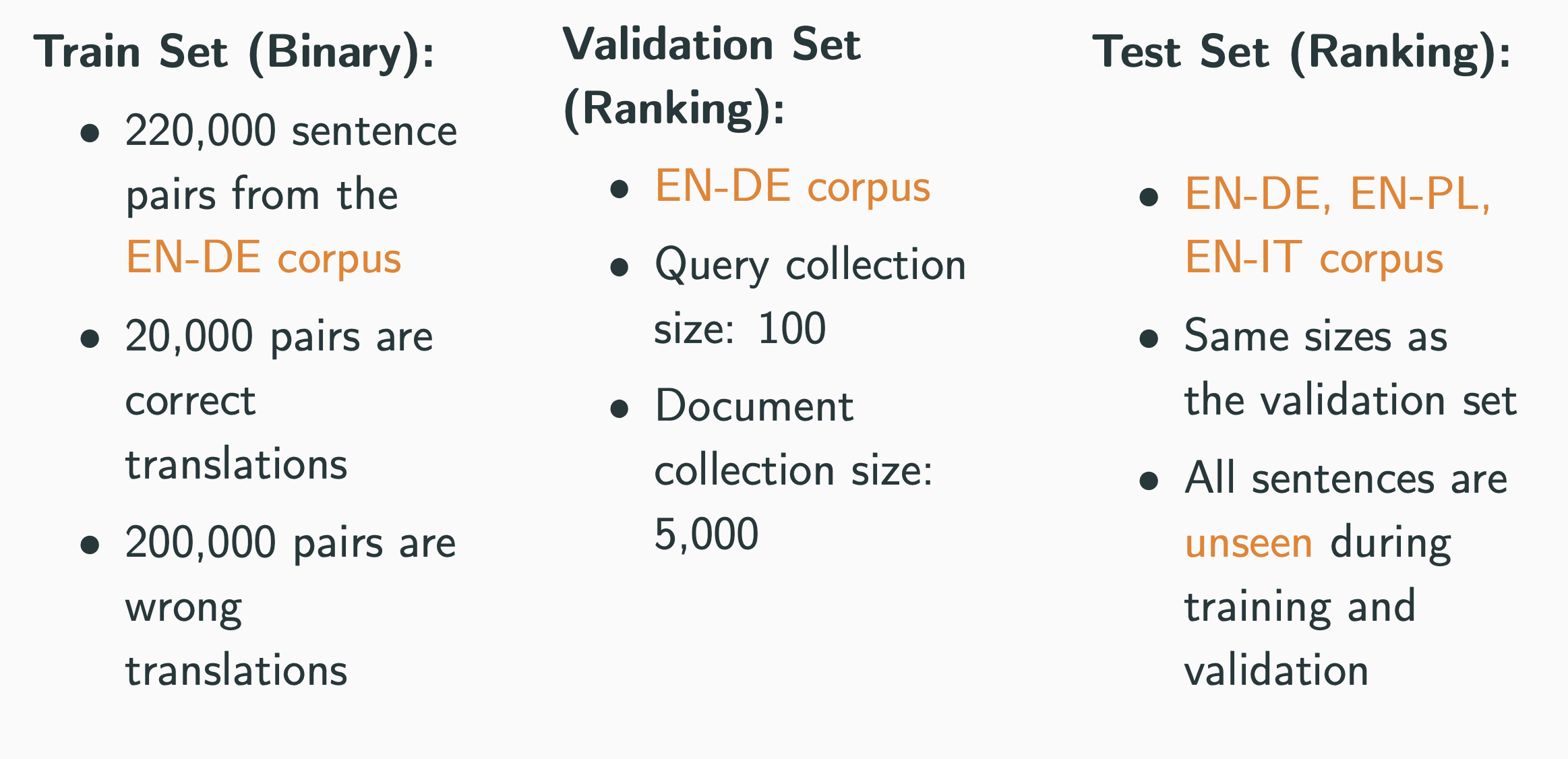 Summary of Train, Validation and Testset.
As we produce a ranking, we need a rank-aware evaluation metric. For that purpose, we calculate the Mean Average Precision (MAP), which simplifies, as we only have one relevant document $d$ each query $q$:
\[MAP = \frac{1}{\vert Q \vert} \sum_{j=1}^{\vert Q \vert} \frac{1}{R_{d_j}},\]where $Q$ is the set of queries and $R_{d_j}$ the rank of the corresponding right translation of query $j$. We always report the MAP score, if not otherwise stated.
3.2.2. Models
In this section, we describe our selected models and show that we improve performance significantly by doing feature and hyperparameter selection (on the validation set). First, we discard correlated features and features that only have one value. We use z-normalization to scale our features and get a first estimator for all models with 97 features in total. To improve our model, we use forward selection for every model to get the best subsets and afterward perform hyperparameter optimization via Grid Search on our validation set. The results of the selection on our validation set can be seen in Table 3.
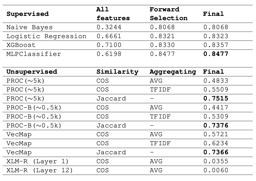 Table 3: For the supervised methods, we evaluate all features and then select a subset of features. Finally, we report our results after hyperparameter-tuning on our validation set (MAP score). Additionally, we report and choose our best unsupervised method.
The final results on our unseen EN-DE test set can be found in Table 4.
Naive Bayes. As we still have many features which could correlate with each other, our Naive Bayes model only achieves a MAP score of 0.3244. However, we can significantly improve the performance up to the 0.8068 MAP score with 12 features when making a forward selection. As there is no hyperparameter for this model to select, we get the final MAP score of 0.8068.
Logistic Regression. Starting from our baseline using all the features, we get a MAP score of 0.6661. We now use forward feature selection to reduce our feature space even further, which results in a MAP score of 0.8321 using only 13 features. In the next step, we use hyperparameter optimization to get an even better estimate. We test different settings, but unfortunately, this only improves our final MAP score by a small margin achieving a final map score of 0.8323 using 14 features, seven of them embedding-based and seven text-based.
XGBoost. XGBoost starts with a MAP score of 0.7100 and is then improved with our forward selection, reaching a MAP score of 0.8330. It only selected three embedding and five text-based features. Unfortunately, we could not increase performance by our hyperparameter optimization significantly, as we could only test a handful of different hyperparameter combinations since we lacked the computational power.
MLPClassifier. For the MLPClassifier, we see that our first baseline performs poorly with a MAP score of 0. 6198 for all 97 features in the default setting (1 hidden layer with 100 hidden units). It seems that the model is too complex and therefore overfitting the train data. So, we use forward feature selection again, resulting in a MAP score of 0.8477 achieved using nine features, 5 of them embedding-based and 4 of them text-based. We try to improve our model performance further using hyperparameter optimization. Trying many different parameter settings, we notice that our model did not improve during the optimization. Surprisingly the default parameter performs best.
 Feature subset sizes after Forward Selection.
XLM-R. To compare our traditional supervised models to transformer models, we choose the massively multilingual transformer model XLM-R. We train the model by using a pre-trained implementation xlm-roberta-base from huggingface (Wolf et al., 2019). We feed the unprocessed sentence pair into the XLM-R tokenizer (seperated by a special token) and then into the model. Our initial experiment shows that the XLM-R model is prone to favor the majority class without any modification and is very unstable, especially at the start of the training. Therefore, to make training more stable, we use a small learning rate at the start and linearly scale it up to the initial learning rate (warm-up steps). We investigate two approaches: In the first one, we downsample the data set to the minority class and randomly sample to create batches (\texttt{XLM-R Downsampling)}. In the second approach, we do not downsample but use the following weighted loss to combat class imbalance:
\[\mathcal{L} = \frac{1}{2} \left(\mathcal{L}\_+ + \mathcal{L}\_\right),\]where $L_+$ is the loss of the positive class and $L_-$ the loss of the negative class. Additionally, we construct a batch, such that it contains the translation and the ten negative translations for each source sentence (XLM-R Weighted).
4. Evaluation
4.1. Evaluation on sentence-level
We are now using our final models both supervised and unsupervised to evaluate our model on an unseen EN-DE test set and perform zero-shot on two different languages: Italian and Polish. With this language combination we have the possibility to judge and compare our performance on languages from different families inside the Indo-European language family, specifically Germanic (DE), Romanic (IT) and Balto-Slavic (PL). Therefore, we use our fitted model trained with EN-DE sentence pairs, on the already mentioned parallel-corpus for English-Italian and EN-PL to get an estimate how suitable our models are for zero-shot transfer. We prepare test sets for both languages that are comparable to our EN-DE test set. Therefore, we create query-document sets with 100 queries and 5,000 documents for the new languages resulting in test sets of 500,000 query-document pairs.
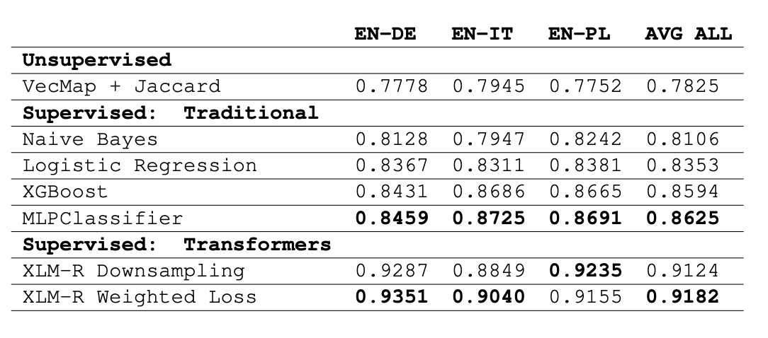 Table 4: Model Comparison on the sentence pair retrieval task. All supervised models were trained on the EN-DE corpus. We show zero-shot performance on EN-IT and EN-PL.
Unsurprisingly, our supervised traditional approaches beat the unsupervised methods. Furthermore, our high MAP scores on Italian and Polish indicate good zero-shot performance, as they are only slightly worse than the MAP scores for German most of the time. In some cases, our model performs even better on the other languages, e.g., the MLPClassifier. Looking at the feature importance of logistic regression and XGBoost, we see that our models put much importance on embedding features that are generated from our embedding spaces, and we noticed in our training process that the alignments work better for EN-PL than for EN-DE. Our best supervised traditional approach is the MLPClassifier with an average MAP score of 0.8625.
The XLM-R with the weighted loss strategy slightly beats the downsampling strategy and achieves the best average MAP score of 0.9182. With these results, we see that using a large, computational demanding XLM-R transformer significantly beats our traditional approaches on the EN-DE and in the other zero-shot languages.
4.2. Evaluation on document-level
Finally, we want to use our trained models on document-level Cross-Lingual Information Retrieval. Therefore, we use the WikiCLIR DE-EN Wikipedia data set (Schamoni et al., 2014) to evaluate whether our models can be used on a document-level task instead of sentence-level.
4.2.1. WikiCLIR data set
The WikiCLIR corpus is a large-scale data explicitly set used for document-level CLIR tasks. It contains 245,294 German sentence queries with 3,200,393 extracted documents from Wikipedia that are marked as either the corresponding English document or another related document. To use our pipeline, we create a test set consisting of 100 queries and 5,000 documents, with 1 denoting the corresponding documents (‘right translation’) and 0 otherwise.
4.2.2. Evaluation
We proceed in the same manner as before and transform the data the same way. As we expected, we can see in Table 5 that all our models perform poorly. We do not get any reliable ranking that can assign the queries to their corresponding documents. Since we use comparable text-based features that are dependent on the comparison between query and documents, we could anticipate this poor performance as they cannot capture the big difference between our sentence queries and the documents. So, our trained models do not have a chance because the training data differs a lot. To get reliable results on document-level, we would need to separately train a model on document-level. Lacking computational power and time, we leave this experiment for future work.
Table 5: Model Comparison for Cross-Lingual Document Retrieval. As we lacked computational power, we do not report the XLM-R Downsampling model.5. Discussion and Outlook
We generated a variety of models to recognize translations and rank documents for queries on sentence-level CLIR tasks. We have seen that using traditional machine learning models can lead to reasonable performances and transmit these results in a zero-shot transfer into other languages. We are sure that more computing power and more training data, especially the MLPClassifier, can be further improved, producing better results. We were, however, not able to beat the XLM-R model. As the gap between our best lightweight model and the XLM-R model is not big, we hypothesize that our models are much more efficient in the retrieval task, and with more time, we could further close this gap, making the high complexity and computational demanding training of XLM-R unnecessary (for this specific task). We also recognize that our models rely heavily on the induced cross-lingual word embeddings and for distant languages, the quality of these embeddings drop (Glavas et al., 2019). Therefore, our supervised methods also suffer in distant languages. However, multilingual transformers also suffer from the same problem (Lauscher et al., 2020). Future work could investigate which method is more robust for distant language pairs. Another aspect one could investigate is, how much the similarity between sentences in the retrieval corpus affect our models. Since we use quite a simple approach, our models could fail in such scenarios, and the transformer model could widen the gap even more. Unfortunately, we can also conclude that our models do not work in any way on document-level tasks. That was to be expected, as we focus a lot on direct comparison features. However, due to the different structures of query and documents in the WikiCLIR data set, these features cannot be transferred in the same manner.
References
Mikel Artetxe, Gorka Labaka, and Eneko Agirre. 2018. A robust self-learning method for fully unsupervised cross-lingual mappings of word embeddings. In Proceedings of the 56th Annual Meeting of the Association for Computational Linguistics (Volume 1: Long Papers), pages 789–798, Melbourne, Australia. Association for Computational Linguistics.
Piotr Bojanowski, Edouard Grave, Armand Joulin, and Tomas Mikolov. 2016. Enriching word vectors with subword information. arXiv preprint arXiv:1607.04606.
Alexis Conneau, Kartikay Khandelwal, Naman Goyal, Vishrav Chaudhary, Guillaume Wenzek, Francisco Guzman, Edouard Grave, Myle Ott, Luke Zettlemoyer, and Veselin Stoyanov. 2020. Unsupervised cross-lingual representation learning at scale.
Alexis Conneau, Guillaume Lample, Marc’Aurelio Ranzato, Ludovic Denoyer, and Herve Jegou. 2018. Word translation without parallel data.
Goran Glavas, Robert Litschko, Sebastian Ruder, and Ivan Vulic. 2019. How to (properly) evaluate crosslingual word embeddings: On strong baselines, comparative analyses, and some misconceptions.
Philipp Koehn. 2005. Europarl: A parallel corpus for statistical machine translation. In Conference Proceedings: the tenth Machine Translation Summit, pages 79—-86.
Anne Lauscher, Vinit Ravishankar, Ivan Vulic, and Goran Glavas. 2020. From zero to hero: On the limitations of zero-shot cross-lingual transfer with multilingual transformers. CoRR, abs/2005.00633.
Robert Litschko, Ivan Vulic , Simone Paolo Ponzetto, and Goran Glavas. 2021. Evaluating multilingual text encoders for unsupervised cross-lingual retrieval.
Chao Xing, Dong Wang, Chao Liu, and Yiye Lin. 2015. Normalized word embedding and orthogonal transform for bilingual word translation. In Proceedings of the 2015 Conference of the North American Chapter of the Association for Computational Linguistics: Human Language Technologies, pages 1006–1011, Denver, Colorado. Association for Computational Linguistics.
Tomas Mikolov, Quoc V. Le, and Ilya Sutskever. 2013. Exploiting similarities among languages for machine translation.
Shigehiko Schamoni, Felix Hieber, Artem Sokolov, and Stefan Riezler. 2014. Learning translational and knowledge-based similarities from relevance rankings for cross-language retrieval. In Proceedings of the 52nd Annual Meeting of the Association for Computational Linguistics.
Peter Schönemann. 1966. A generalized solution of the orthogonal procrustes problem. Psychometrika, 31(1):1–10.
Thomas Wolf, Lysandre Debut, Victor Sanh, Julien Chaumond, Clement Delangue, Anthony Moi, Pierric Cistac, Tim Rault, Remi Louf, Morgan Funtowicz, and Jamie Brew. 2019. Huggingface’s transformers: State-of-the-art natural language processing. CoRR, abs/1910.03771.