The Github Repository can be found here.

Table of Contents

1. Motivation
2. Prerequisite
   1. Route Criteria
   2. Street Network as an undirected Graph
   3. Eulerian Graph
3. Approach
   1. Algorithms for the determination of Eulerian Cycle in Eulerian Graphs
   2. Connecting odd nodes
   3. Final Algorithm
4. Implementation and Simulation Results
   1. Testing the algorithms on an example
   2. Optimal Route in Gartenstadt (Mannheim)
5. Conclusion and Outlook

1. Motivation

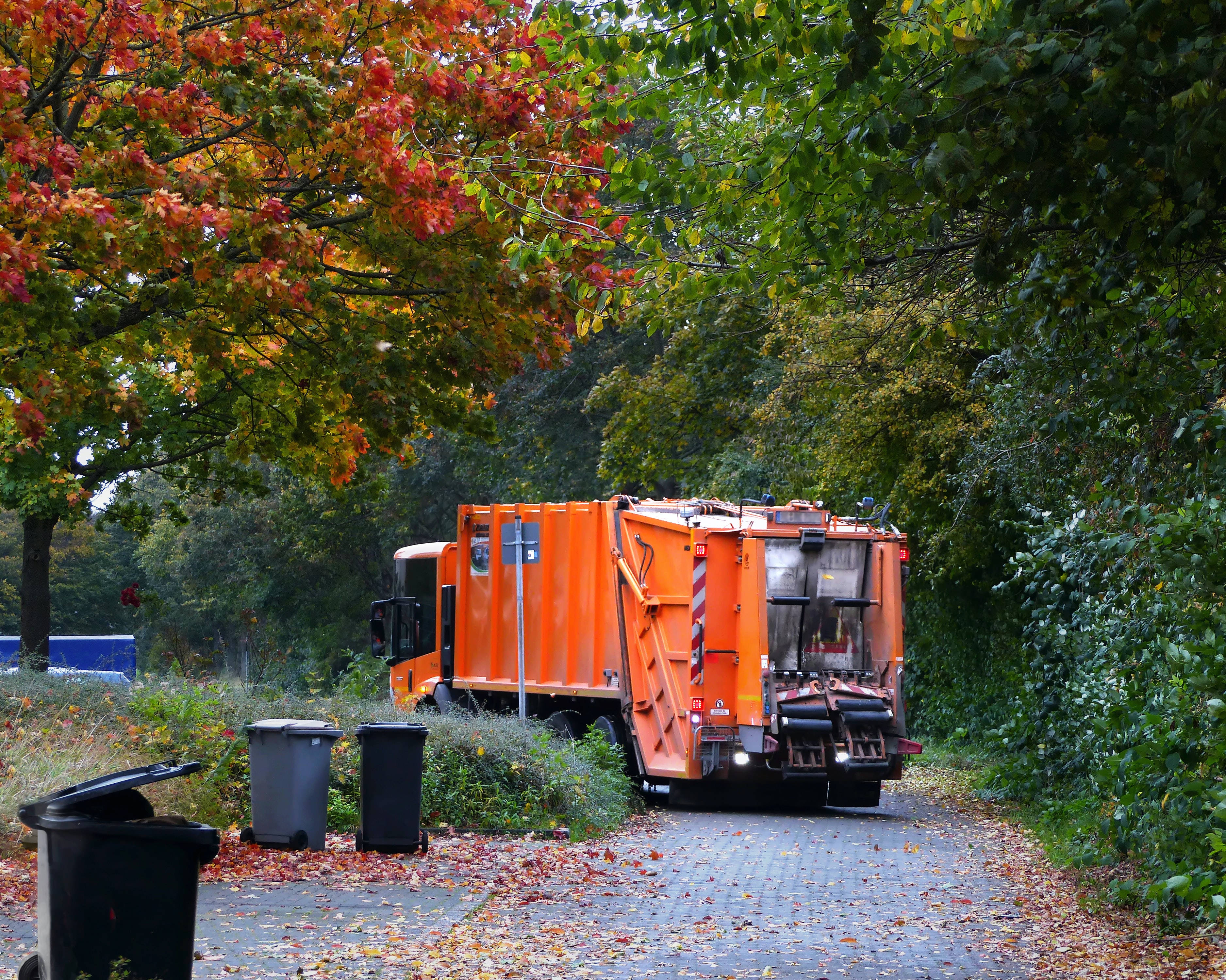
Every city generates waste that has to be disposed of. Each trip by the waste collection service incurs costs, most of which depend on the travel time. To minimize cost, one has to find the fastest possible route. But how can this be calculated?

In Mannheim alone, 108,269 tons of waste (organic waste, green waste and paper) from private households and businesses were disposed of, which means 355 kg/inhabitant and year or about 500 tons daily! At the end of this project we want to create an optimal route for the waste collection in a district in Mannheim to minimize the costs of waste disposal.

2. Prerequisite

2.1 Route Criteria

When creating a route for waste collection, various criteria must be met:

• All streets must be used only once (at least), since garbage trucks can dispose of garbage on both sides of the street at once.
• Consider one-way streets and dead ends, which are used in both directions.
• The last criterion should be that our garbage vehicle travels from the garbage dump and back to the same garbage dump, that is, the starting point and ending point of the trip should be the same.
• We assume that we have only one garbage vehicle, so we have to assume that we have a road network where we can reach every road.
• In this project, we will only consider road networks that do not have one-way roads in order to simplify our mathematical model.

2.2. Street Network as an undirected Graph

Each edge in an undirected graph can only ever run in both directions. With such edges we can therefore represent any road in our model, since we do not allow one-way roads that may only be traveled in one direction. We additionally assume that our undirected graph, is contiguous, i.e. any node must be reachable by any other node, since we have only one garbage truck, which must travel all roads.

Each node is modeled as an intersection or as a dead end. This allows us to represent each road network in our simplified model as a connected undirected graph.

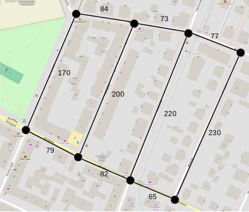
We can now further specify our model by assigning edge weights so that we can represent different types of variables, such as road lengths, travel time or road processing time. The reason for the specification is that we cannot always find a route that travels each road only once and thus we have to travel roads twice. As a result, routes can differ if we want to minimize either the path length or the travel time. But since we have to dispose the garbage exactly once for each road, we can ignore the processing time. Thus, the edge weights in Fig. 1 can represent the travel time.

2.3. Eulerian Graph

So our problem now is: Find an optimal path that minimizes the sum of the weights from the edges, runs through each edge at least once, and whose starting point and ending point are identical.

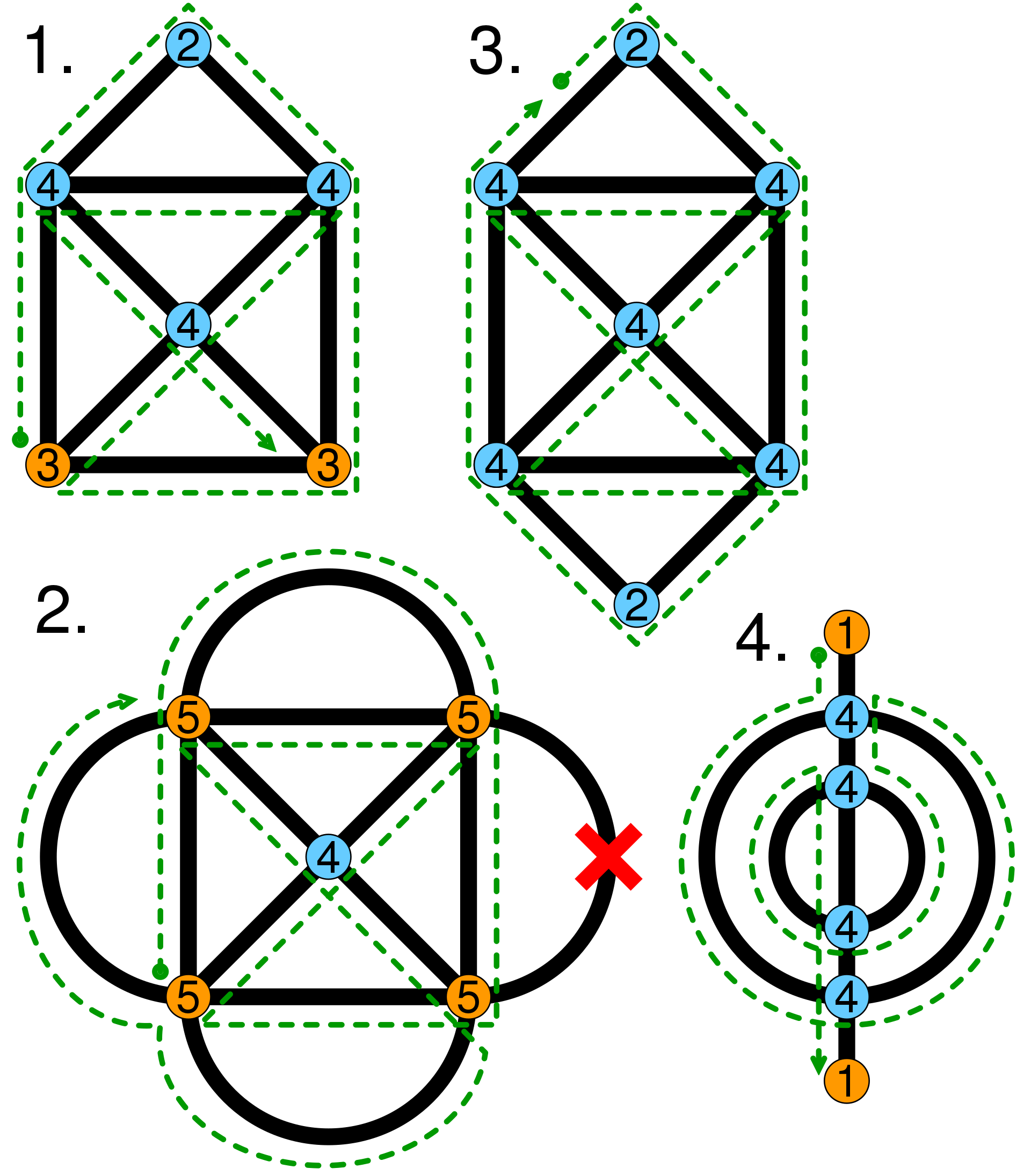
A path which runs through each edge in our graph exactly once, but which does not yet satisfy the condition that the start and end points are the same, is also called an Eulerian path. However, since in our model the starting point should be equal to the end point, our Euler path must also be a circle. A circle is a path whose starting and end points match. This special Eulerian path is also called an Eulerian cycle.

Definitions. An Eurelian graph is a graph with an Eulerian circuit. An Eulerian circuit or Eulerian cycle is an Eulerian trail that starts and ends on the same vertex. An Eulerian trail (or Eulerian path) is a trail in a finite graph that visits every edge exactly once (allowing for revisiting vertices).

Thus, if we can find an Eulerian cycle that minimizes the sum of the weights on the path, then we have found an optimal Solution to our problem!

Solution

The most important theorem to answer our question whether there exists an Euler cycle in a graph had already been formulated by Euler (1736) for his famous Königsberger Brückenproblem. With this theorem we can characterize all Eulerian graphs:

Theorem. A connected graph is Eulerian if and only if each vertex has an even degree (=number of edges connecting it).

3. Approach

3.1. Algorithms for the determination of Eulerian Cycle in Eulerian Graphs

In this section we will learn two different algorithms to find an Euler tour on an Eulerian graph, knowing now that the graph is connected and has only nodes with even degree. The property will come in handy to prove the correctness of the algorithms.

Hierholzer’s Algorithm

The algorithm was published by the mathematician Carl Hierholzer in 1871. The idea of the algorithm is to gradually decompose the entire graph into different circular graphs, which are then combined to form an entire circle. Formally, the process can be divided into 3 steps:

1st Step:

• Choose any starting node v0
• Choose unvisited edges until the starting node is reached again. The constructed path is a circle K.

2st Step:

• If K is an Euler tour, break off and K is our Solution. Otherwise go to step 3.

3st Step:

• Set K’=K.
• Choose node w from the circle K’ which has an unvisited edge.
• As in the 1st step, construct for w a circle K’’ , where we consider only the graph without edges from the circle K’.
• Now we want to reconstruct the circle K by containing the circles K’ and K’’ : Go from v0 in K’ along K’ to the node w. Then traverse the new circle K’’ once completely and, arriving back at w, traverse the rest of K’. Denote this path as K.
• Go to step 2.

Fleury’s Algorithm

Another algorithm for determining the Euler tour is Fleury’s algorithm. In contrast to Hierholzer’s algorithm, this algorithm does not interrupt the construction of the tour. The algorithm draws “without putting down the pen”, but it is also slower than Hierholzer’s algorithm. Before we can understand the structure of the algorithm, we have to introduce the term bridge, because it plays an important role in the algorithm.

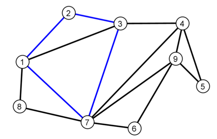
Definition (Bridge). A bridge is an edge e whose deletion would decompose the graph into two components.

If all node degrees in a graph are even, then it has no bridges. So we know that if we have an Eulerian graph, then it has no bridges. Fleury’s algorithm is constructed on the basis of this fact. The algorithm gradually extends an empty path to the beginning until it is an Eulerian tour.

1st Step:

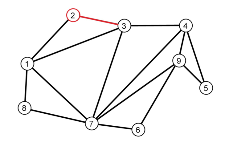
• Start with an arbitrary starting node and select an incidenced edge.

2st Step:

• Select the next unvisited edge. The edges to be selected are those that satisfy the 2 conditions, where the 2nd condition may be violated if there are no other edges that satisfy it:
  1. incident to the last visited edge.
  2. edge (u, v) is not a bridge in the residual graph consisting of all edges not yet visited. We u ̈verify this condition by searching for a (u, v)-path in the residual graph without the edge (u, v). If we can find such a path, e.g., with depth-first search, then we know that the edge must be a bridge, because we can extend the found path (u, v) to a circle with the edge u, v. But an edge is not a Bru ̈cke if it lies on a circle!

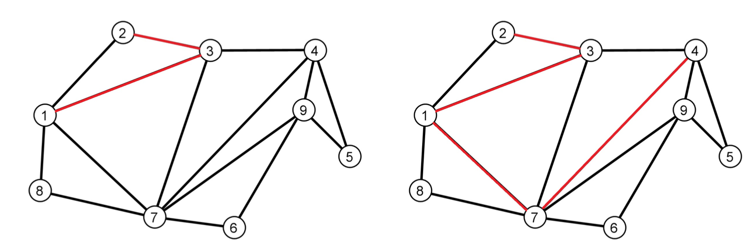
Summary.

We now know two different algorithms to find an Eulerian tour in an Eulerian graph. The only problem that remains is: Our road network does not have to be an Eulerian graph! Sure, because not every intersection has an even number of roads, i.e. we have nodes that have an odd degree.

3.2. Connecting odd nodes

We look in this section at the case when the graph has odd nodes. We first note that there exists no graph that has an odd number of nodes with odd degrees. From this follows the theorem:

Theorem. In every graph the number of nodes with odd degree is even.

The idea now is to connect the nodes with odd degrees in pairs, where we want to connect them in the shortest way to minimize the sum of edge weights. This works for any non-Eulerian graph, since we know that it always has an even number of nodes with odd degrees. If the connection passes through other nodes with even degree, their degree always increases by 2 as the edge leads in but also leads out of the node. By connecting nodes with odd degrees, we have now created a graph consisting only of nodes with even degrees.

We will use Dijkstra’s algorithm to find a shortest connection between 2 odd nodes.

3.3. Final Algorithm

1. Convert the road network into an undirected connected graph, where intersections are the nodes and roads are the edges, and dead ends are ignored for now.
2. If the graph has nodes with odd degrees, then consider these nodes and find a connection with the smallest sum of edge weights (using Dijkstra’s algorithm) to keep our route optimal.
3. Insert the connection in the form of edge moves in the graph.
4. In the case of dead ends, we have to go in and out. So for dead ends, double edges are drawn in.
5. We now have an Euler graph and each Euler tour is optimal. We can apply our algorithms from Hierholzer and Fleury to find an Euler tour. Now we have found an optimal route and we are done!

4. Implementation and Simulation Results

4.1. Testing the algorithms on an example

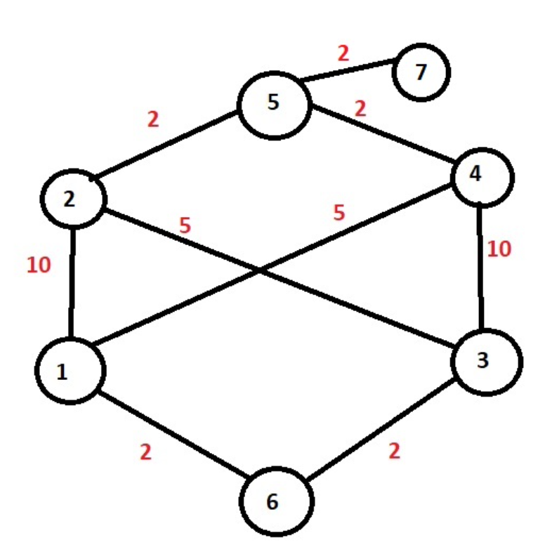
1st Step:

We will first determine the dead ends of the graph with the function “dead end”. Now we can find the corresponding edges in the incidence matrix.

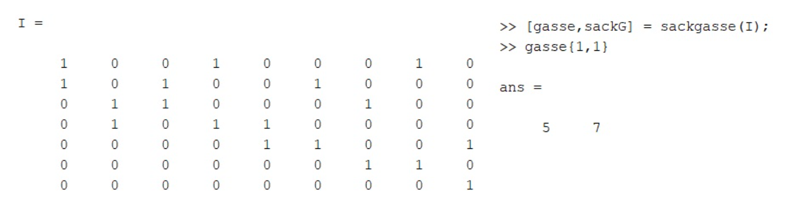
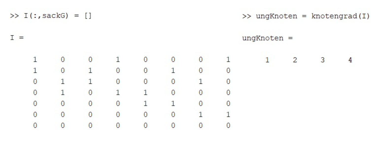
2st Step:

Our present graph obviously has nodes with odd degree, so we need to convert the graph into an Eulerian graph, i.e. a graph with only even node degree. So the first thing we need to do is find all the nodes with odd degree. This can be done with the algorithm “node degree”.

Now we want to find a minimal matching for the nodes with odd degrees. For this purpose I wrote the function “minMatchin”, which is based on “maxWeight Matching” by Daniel Saunder4. We want to modify his function so that we can calculate a minimum matching given for certain points in a graph. The problem of the function “maxWeightMatching” is # that it calculates a maximum matching for all nodes in the graph.

In our case, however, we want to calculate a minimum matching given for certain nodes, namely the odd nodes, in a graph.

Idea: Converting a maximal matching into a minimal matching is easy, we reverse all signs of our edge weights. Obviously, if we apply the maximal matching to the edges with the new weights, we get a minimal matching. The problem remains that we only want to consider certain points.

We first make the following consideration: We compute ALL paths that exist between all odd nodes. We perform (mentally) the minimal matching we are looking for odd nodes only. If we now look at 2 previously odd nodes a and b that have been connected, then the minimal matching must have chosen one of the paths that we have previously calculated, since we have finally calculated all the paths between a and b that exist. The crucial thing is that no path is dropped in the course of matching, i.e., if we have connected two nodes, we can still run any existing path to connect the other nodes. So we can model all paths between all odd nodes as one edge with corresponding edge weights!

Matching will of course then see no difference than if we consider the paths as individual edges, as long as the edge weights match. So we can confidently run our matching over the new edges. The problem with this method is that we need a very high computational cost, since we need to compute all paths between all odd nodes. That’s why I looked for another way to solve the problem:

We consider the approach from above and modify it. We calculated all possible paths and modeled them as edges, but it follows that all paths between 2 nodes are modeled as parallel edges. Minimal matching will, of course, select only the most minimal edge between 2 nodes! On our original graph, this now means that we have chosen the shortest path between a and b. We can use Dijkstra to compute all shortest paths between all odd nodes and model these paths as edges in the new graph, rather than all mo ̈possible paths. We then apply minimal matching to this and, of course, at the end we have to transform the selected edges back into a path in the old graph.

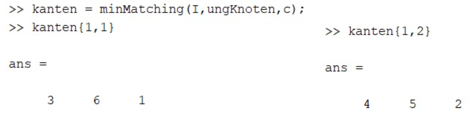
3st Step:

We add the found edge features to our road mesh using the “kantenhinzufugen” function.

4st Step:

The last step to obtain an Eulerian graph is to represent the dead ends by double edges. Adding these edges is done again with “kantenhinzufugen”, where we have to add twice, because we deleted the dead ends in the 1st step.

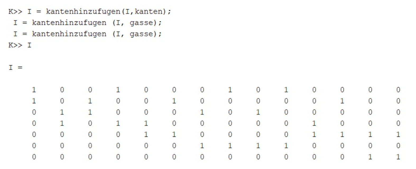
5st Step:

We now have an Euler graph and can run our 2 algorithms.

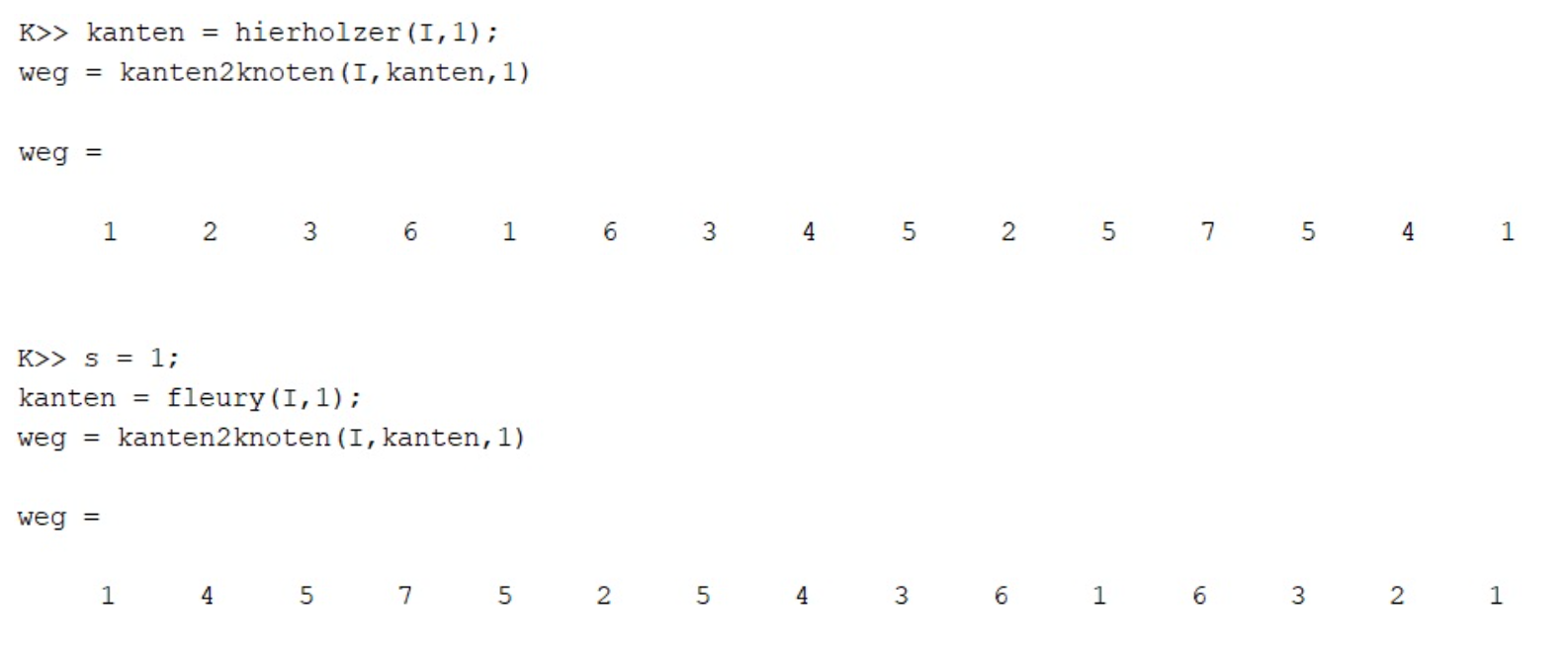
We can easily see with a drawing of the path in the graphs that the two paths must be the optimal path.

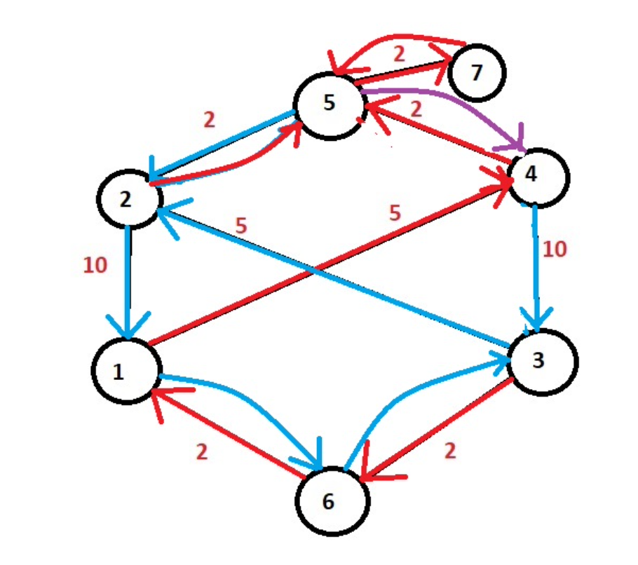
4.2. Optimal Route in Gartenstadt (Mannheim)

In this section, we will construct an optimal route planning for garbage collection for a street network of Mannheim. For this purpose, we take the district “Gartenstadt” in Mannheim, since it contains only one street that our model does not take into account, namely a street that has to be traveled twice. We can ignore this and the road network is thus suitable for our simplified model

First, we delimit the district and choose a starting node for which we want to find an optimal route by applying our elaborated scheme.

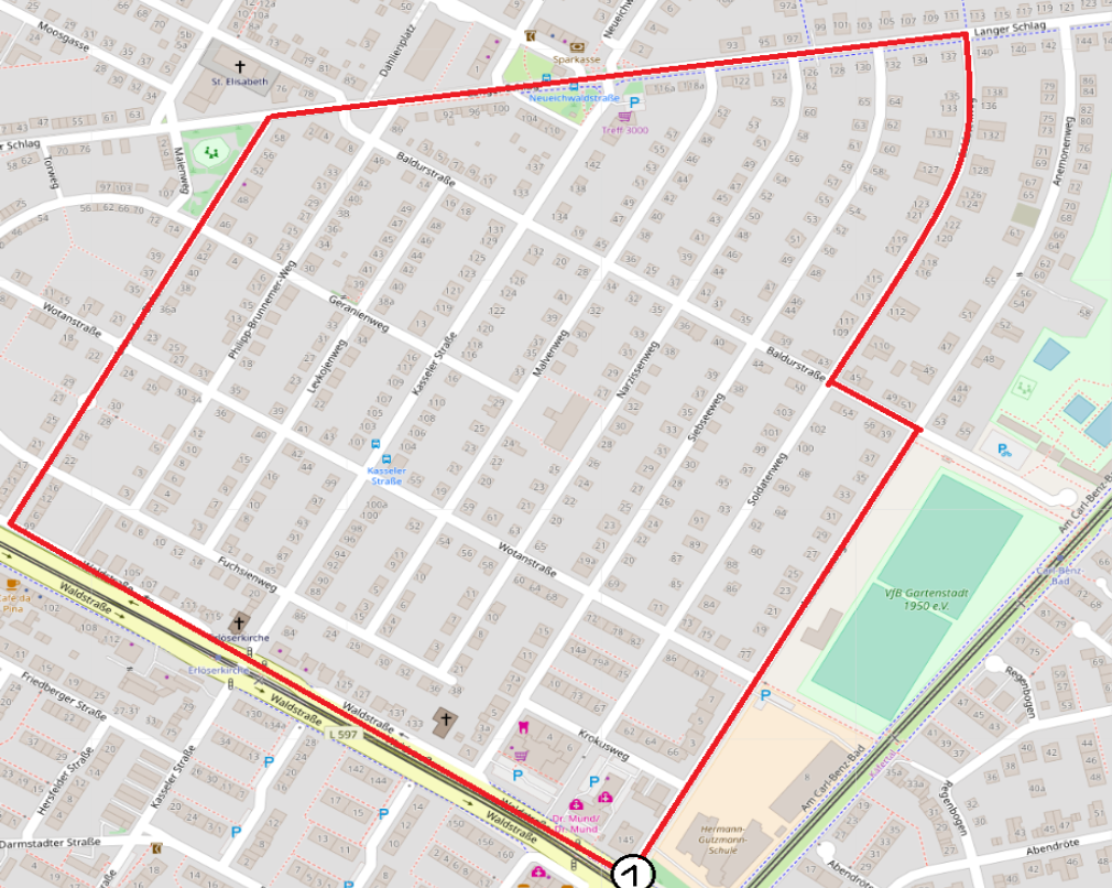
1st Step:

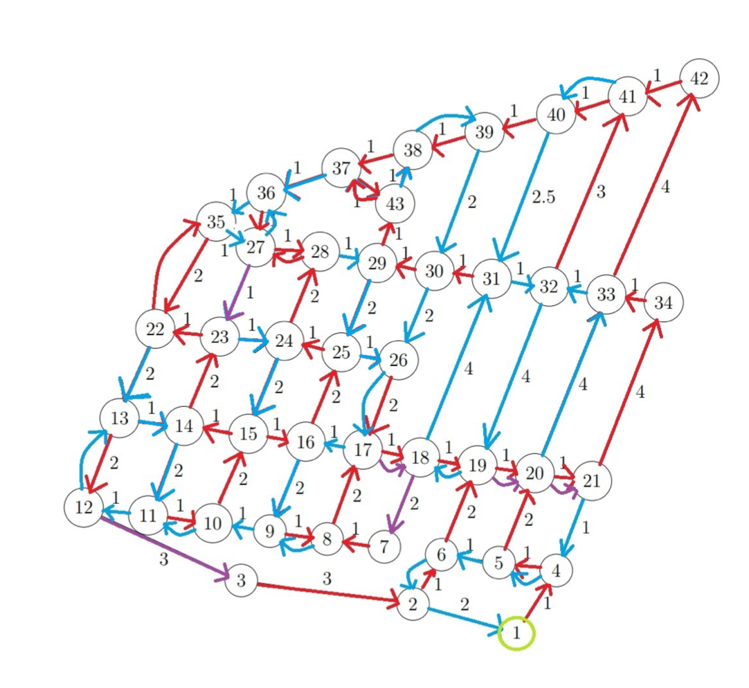
Convert the road network into a graph. The numbers on the edge are not the edge weight but just a numbering.

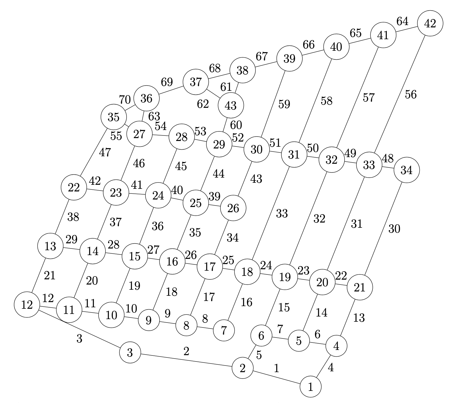
First, we build the incidence matrix using the algorithm “incidencematrix”, which creates an incidence matrix from a string drawing a graph in latex. Next, we assign edge weights to each edge. Here, we want to take time as the edge weight, with the given times rounded up and measured by Google Maps.

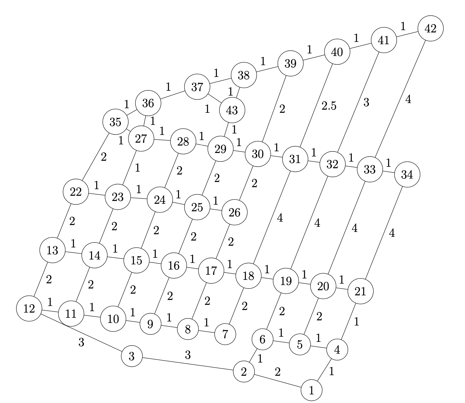
Now we can go through the individual steps analogously as in the 1st example. Our final result then looks like this:

5. Conclusion and Outlook

No model that is supposed to reflect reality is perfect. We can still do some things to make our model more realistic. Even at the very beginning, our model included restrictions: One-way streets and streets that must be traveled twice. An extension of the model with these two constraints could be done.

In addition, we did not take into account that garbage trucks naturally cannot pick up an infinite amount of garbage, i.e., they have to go back to the dump to unload once they reach a certain capacity. This will of course make our problem more complex.